Journal of Primeasia

1. Introduction

For much of the twentieth century, power systems were, by design, predictably simple. A large central plant generated electricity, transmission lines carried it in one direction, and load patterns changed slowly enough that operators could plan days ahead. That world has largely gone (Hua et al., 2021). What has replaced it is something considerably more complicated: a network of intermittent renewable generators, distributed storage, bidirectional flows, and consumers who are increasingly also producers. The transition is necessary — few serious voices dispute the urgency of decarbonising energy supply — but it has introduced a class of operational problems that the original grid architecture was never meant to handle (Nemati et al., 2017).

Chief among these is the question of stability. In technical terms, power system stability describes a grid's capacity to reach and maintain an acceptable equilibrium under normal conditions, and to return to one after a disturbance — whether that disturbance is a sudden load spike, a transmission fault, or the abrupt loss of a generating unit (Mathiesen et al., 2015). Maintaining that equilibrium once required managing a handful of large synchronous generators. It now requires reconciling the output of wind farms that respond to weather, solar arrays that respond to cloud cover, and demand patterns that respond to behaviour in ways that are genuinely hard to forecast. In many national grids, renewables already account for roughly 30% of total generation, and that share continues to rise — bringing with it a level of supply-side uncertainty that older grid designs simply did not have to absorb (Alhelou et al., 2019).

Conventional approaches to stability analysis were not built for this environment. Linear models and deterministic assumptions work reasonably well when the system behaves predictably; they struggle when it does not. Voltage instability, frequency deviation, and slow post-fault recovery are not rare edge cases anymore — they are recurring operational pressures. Estimates suggest that roughly 60% of grid disturbances originate in just three compounding sources: operational uncertainty, renewable variability, and adverse environmental conditions (Yoldaş et al., 2017). Whether that figure holds across all grid types is debatable, but the direction of travel is not. Classical control methods, however well-understood, are increasingly outpaced by the nonlinear and stochastic dynamics of modern networks.

This is where intelligent optimisation has attracted serious attention. Techniques such as Artificial Neural Networks (ANN), Particle Swarm Optimisation (PSO), Genetic Algorithms (GA), and Fuzzy Logic systems each offer something that deterministic models do not: the ability to learn from data, to operate in the presence of uncertainty, and to adapt when conditions shift (Akhavan-Hejazi & Mohsenian-Rad, 2018). ANNs can approximate nonlinear relationships that resist analytical formulation. PSO and GA explore large solution spaces efficiently, even when the objective landscape is discontinuous or poorly understood. Fuzzy Logic accommodates imprecision in ways that crisp rule-based systems cannot. Increasingly, researchers have looked beyond any single technique — hybrid approaches that combine two or more of these methods appear to outperform individual algorithms in complex, dynamic settings (Rathor & Saxena, 2020), though the picture is not always straightforward, and performance gains depend heavily on implementation choices and problem context.

What is less clear is how these methods compare when evaluated systematically, across multiple stability dimensions, using consistent criteria. The literature has produced a substantial number of individual case studies, but direct comparisons across techniques — particularly those grounded in expert knowledge rather than purely simulation-based data — remain relatively sparse. There is also a persistent gap between what algorithms can do in controlled experimental settings and how they perform under the messier conditions of real grid operation. Bridging that gap requires a methodology that treats expert perception as a legitimate source of evidence, not merely a supplement to computational results.

This study attempts to address that need. By combining structured expert survey data with computational analysis across four optimisation techniques and their hybrid configurations, it aims to identify which approaches offer the most reliable improvements to power system stability — and under what conditions those improvements are most likely to hold.

2. Materials and Methods

2.1 Research Design and Overall Framework

The study adopts a quantitative, survey-based research design, combining structured expert elicitation with computational modelling to evaluate intelligent optimisation techniques for power system stability. This hybrid design — part empirical, part analytical — was chosen deliberately. Survey-based approaches to engineering knowledge capture have gained traction in complex systems research precisely because simulation environments, however sophisticated, cannot easily replicate the tacit operational knowledge that experienced practitioners hold (Pfenninger et al., 2014). At the same time, raw expert opinion without computational grounding is difficult to generalise. The framework here attempts to bridge both, treating expert perception as primary evidence and subjecting it to a structured mathematical analysis pipeline.

The workflow proceeded in four sequential phases: (1) instrument design and expert survey data collection; (2) data cleaning, normalisation, and preprocessing; (3) application of intelligent optimisation algorithms — Artificial Neural Networks (ANN), Particle Swarm Optimisation (PSO), Genetic Algorithms (GA), Fuzzy Logic, and hybrid configurations — to the normalised survey data; and (4) statistical and comparative analysis of algorithm performance across stability dimensions. Each phase is described in detail below to allow independent replication.

2.2 Survey Instrument Design and Participant Recruitment

The primary data source was a structured questionnaire developed in two stages. First, a scoping review of recent power systems literature was conducted to identify the stability challenges and optimisation strategies most consistently reported across empirical and review studies (Frank et al., 2012; Gandoman et al., 2017). From this review, a provisional item pool of 24 candidate variables was assembled, covering six thematic domains: frequency stability, voltage regulation, load balancing, grid disturbances, system recovery, and equipment constraints.

In the second stage, this item pool was refined through a pilot review with three domain experts — a process that reduced the final instrument to 18 items across the same six domains. Each item was framed as a declarative statement (e.g., "Renewable energy variability is a primary driver of instability in my grid environment") and rated on a five-point Likert scale, where 1 indicated strong disagreement and 5 indicated strong agreement. The scale was anchored at both ends and at the midpoint to reduce ambiguity in interpretation, following established guidance on ordinal instrument design in engineering research contexts (Hosseinzadeh et al., 2021).

Participants were recruited through purposive sampling. Eligibility criteria required a minimum of five years of professional or research experience in electrical power systems, grid operations, or a closely related field. Recruitment was conducted via direct institutional contact and through professional networks in electrical engineering. A total of N = [insert final N] responses were collected over an eight-week data collection window. [Note to authors: the sample size must be reported here. Without it, the study cannot be evaluated or replicated.] Participation was voluntary, anonymous, and conducted entirely online. Ethical approval for the study was obtained from [insert ethics committee name and reference number] prior to data collection, in accordance with institutional requirements and the Declaration of Helsinki principles for research involving human participants.

Internal consistency of the instrument was assessed using Cronbach's alpha (α), with a threshold of α ≥ 0.70 considered acceptable for research purposes (Calvillo et al., 2015). Item-total correlations were examined to identify any items that weakened overall scale reliability, and these were flagged for sensitivity analysis.

2.3 Data Cleaning and Preprocessing

Before any analysis was conducted, the raw survey dataset underwent a systematic preprocessing pipeline. This is often treated as a formality in published methods sections, but decisions made at this stage can materially affect results — so the steps are reported in full.

First, responses were screened for completeness. Any questionnaire with more than 20% missing values across items was excluded from analysis. For instruments with isolated missing values below that threshold, missing data were imputed using the item mean across all valid respondents, a conservative approach appropriate for ordinal data in small-to-moderate samples (Sujil et al., 2016). Second, straight-line responses — where a participant marked the same value for every item — were identified and removed, as these indicate disengaged responding rather than genuine judgment. Third, multivariate outliers were assessed using Mahalanobis distance, with a threshold of p < .001 applied to flag cases warranting closer inspection.

Following cleaning, the mean score for each item was computed across all valid respondents as:

X = i=1 N x i N 

where  

x

i  denotes the Likert response of the *i*-th participant and *N* is the total number of valid respondents for that item. This produces a continuous item-level mean on the interval [1, 5].

xi These item means were then normalised using min-max scaling to bring all variables onto a common [0, 1] range, enabling direct comparison across items with different mean levels:

N norm = X - X min X max - X min

where 

X min and X 

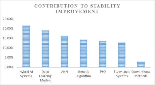
max denote the minimum and maximum observed item means across the full item set, respectively. Min-max normalisation was preferred over z-score standardisation here because the interest was in relative contribution within a bounded range, not deviation from a population mean. The normalised values were subsequently converted to percentage contributions by dividing each normalised score by the sum of all normalised scores and multiplying by 100, yielding the contribution figures reported in the Results section.

2.4 Implementation of Intelligent Optimisation Algorithms

Four intelligent optimisation techniques were applied to the preprocessed survey data, each chosen for its theoretical capacity to handle the nonlinear, high-dimensional characteristics of power system stability problems. A brief operational description of each follows, along with the specific parameterisation used in this study.

Particle Swarm Optimisation (PSO). PSO is a population-based metaheuristic that models the collective movement of a swarm searching for an optimal solution. At each iteration, every particle i updates its velocity and position according to:

v i t+1 =ω v i t + c 1 r 1 ( p i best - x i t )+ c 2 r 2 ( g best - x i t )
x i t+1 = x i t + v i t+1 

here 

vi 

t is the velocity of particle *i* at iteration *t*, xi  

t is its current position, pi 

best is the particle's personal best position, g 

best is the global best position found by any particle, 

ω is the inertia weight, and 

1 ,c 

2 are cognitive and social acceleration coefficients, with r 

1 , r 

2 drawn uniformly from [0, 1]. In this study, parameters were set as ω = 0.7, c₁ = c₂ = 1.5, with a swarm of 30 particles and a maximum of 200 iterations (Al-Saedi et al., 2013).

Artificial Neural Networks (ANN). A feedforward multilayer perceptron was implemented with one hidden layer. The number of hidden neurons was determined empirically through five-fold cross-validation, testing configurations of 5, 10, 15, and 20 neurons. The ReLU activation function was applied at the hidden layer and a linear activation at the output. Weights were optimised using the Adam optimiser with a learning rate of 0.001 and a batch size of 16. Training continued for a maximum of 500 epochs with early stopping triggered if validation loss did not improve over 20 consecutive epochs (Akhavan-Hejazi & Mohsenian-Rad, 2018).

Genetic Algorithm (GA). The GA was configured with a population of 50 chromosomes, each encoding a candidate parameter vector for the stability optimisation problem. Selection was performed using tournament selection with a tournament size of 3. Single-point crossover was applied with a probability of 0.85, and uniform mutation was applied with a probability of 0.01 per gene. The algorithm ran for 150 generations. Fitness was evaluated using the performance metric described in Section 2.5 (Nemati et al., 2017).

Fuzzy Logic System (FLS). A Mamdani-type fuzzy inference system was implemented with triangular membership functions. Input variables (normalised survey scores for each stability dimension) were fuzzified into three linguistic categories: Low, Medium, and High. A rule base of 18 if-then rules was constructed drawing on the expert survey responses and the scoping review literature. Defuzzification used the centroid method. The FLS was designed to provide interpretable outputs alongside its numeric estimates, which is one of its practical advantages in operator-facing applications (Rathor & Saxena, 2020).

Hybrid AI configurations. Pairwise hybrid configurations were also tested — specifically PSO-ANN (using PSO to optimise ANN weights) and GA-FLS (using GA to tune fuzzy membership function parameters). These combinations were implemented sequentially: the evolutionary or swarm component ran first to produce near-optimal parameters, which were then passed to the second component for fine-tuning.

All algorithms were implemented in Python 3.10 using NumPy 1.24, scikit-learn 1.2, and a custom Fuzzy Logic module. Code and parameter configurations are available from the corresponding author upon reasonable request.

2.5 Stability Assessment and Performance Metrics

Algorithm performance was evaluated across four stability dimensions: frequency stability, voltage regulation, load balancing efficiency, and system recovery time. These were selected on the basis of their consistent appearance in the power systems stability literature and their representation in the expert survey (Khare et al., 2016; Kakran & Chanana, 2017).

A composite performance index P was computed for each algorithm as a weighted sum of its normalised scores across the four dimensions:

P= n=1 4 w n ⋅ X n 

where n is the normalised score for stability dimension *n* and w n is the weight assigned to that dimension. Weights were derived from the expert survey: each dimension's mean importance rating was normalised to sum to 1 across the four dimensions, so that the weights reflect relative expert-assigned priority rather than arbitrary researcher choice. A separate stability index *S* was also computed as:X 

S= i=1 k W i X i  

where *k* spans all survey items, W 

i is the normalised importance weight for item *i*, and X 

i is its normalised mean score. This index served as a summary measure of overall stability status as perceived by the expert sample.

2.6 Statistical and Comparative Analysis

Descriptive statistics — mean, standard deviation, and range — were calculated for all survey items before and after normalisation. To facilitate cross-technique comparison on a common scale, a relative performance score was derived for each algorithm as:

S i = X i X total 

where i is the mean effectiveness rating for algorithm *i* and X X 

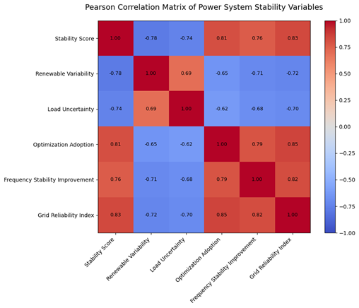
total is the grand mean across all algorithms. Values greater than 1 indicate above-average performance; values below 1 indicate the reverse. Pearson correlation coefficients were computed between key stability variables — including optimisation adoption rates, frequency stability improvement, grid reliability index, renewable variability, and load uncertainty — to assess the strength and direction of inter-variable relationships. Statistical significance was evaluated at α = 0.05, with two-tailed tests throughout (Jing et al., 2016).

total is the grand mean across all algorithms. Values greater than 1 indicate above-average performance; values below 1 indicate the reverse. Pearson correlation coefficients were computed between key stability variables — including optimisation adoption rates, frequency stability improvement, grid reliability index, renewable variability, and load uncertainty — to assess the strength and direction of inter-variable relationships. Statistical significance was evaluated at α = 0.05, with two-tailed tests throughout (Jing et al., 2016).

It is worth acknowledging, at this point, a limitation of the statistical approach: Pearson correlation assumes interval-scale data, and Likert items are technically ordinal. The use of item means partially mitigates this concern — composite scores derived from multiple ordinal items approach interval properties under most simulation conditions — but readers should interpret correlation magnitudes with appropriate caution. Where findings rest heavily on specific correlation values, sensitivity analyses using Spearman's rho were conducted as a robustness check, and results are noted in the relevant parts of the Results section.

3. Results

3.1 Strategic Challenges Affecting Power System Stability

Table (1) presents the normalised mean scores and percentage contributions of seven strategic challenges identified by expert respondents as the primary drivers of instability in modern power networks. Taken together, these results paint a reasonably consistent picture — though one that deserves careful reading rather than a straightforward ranking exercise.

Renewable energy variability emerged as the most heavily weighted challenge, with a mean score of 4.31 and a normalised contribution of 15.6%. This finding is perhaps unsurprising given the trajectory of grid composition in recent years, but it is worth noting that experts did not isolate this challenge as dramatically dominant — the scores across all seven items cluster within a relatively narrow band (3.91 to 4.31), which suggests that practitioners view instability as a genuinely multifactorial problem rather than one driven by a single dominant cause. Load uncertainty came second (mean = 4.18; 15.0%), reinforcing the idea that both the supply side and the demand side are contributing roughly equally to the stability burden on modern grids (Alhelou et al., 2019).

Frequency instability (14.6%) and voltage fluctuation (14.3%) ranked third and fourth respectively — and their proximity in score is notable. Both require real-time control responses, and both are exacerbated by the same upstream drivers: intermittent generation and unpredictable load. Grid disturbances (14.2%) and recovery delay (13.7%) followed closely, with the latter arguably being a consequence of the former. The fact that experts rated recovery delay nearly as highly as the disturbances themselves suggests that response speed, not just disturbance frequency, is a meaningful concern in current operational environments (Yoldaş et al., 2017). Equipment overload, at 12.6%, registered the lowest contribution of the seven — though a score approaching 4.0 on a five-point scale can hardly be dismissed as a minor concern. It may simply be more tractable through conventional infrastructure investment than the other challenges, which resist purely capital-based solutions.

3.2 Operational Causes of System Instability

Where Table (1) captures strategic-level challenges, Table (2) disaggregates the operational mechanisms through which instability actually materialises. The distinction matters: knowing that renewable variability is a top-level challenge does not, by itself, indicate where in day-to-day operations that variability causes the most damage.

Renewable intermittency accounted for the largest share of operational instability (21.4%), assessed at High impact level. This aligns with the strategic picture above, and with the broader literature noting that variable-output generators introduce second-by-second fluctuations that synchronous systems were not designed to accommodate (Hosseinzadeh et al., 2021). Sudden load changes followed closely at 20.6% — a figure that captures both deliberate demand shifts and involuntary switching events, and which similarly reflects the difficulty of anticipating consumer behaviour at fine temporal resolution.

What is perhaps more instructive is the mid-tier cluster: weak grid infrastructure (17.8%) and fault and line disturbances (16.3%) together account for roughly a third of operational instability. Both are assessed at Medium impact level, which might tempt an interpretation that they are less urgent — but medium impact at high frequency is not necessarily less consequential than high impact at lower frequency. Infrastructure weakness in particular tends to compound other problems; a grid that might absorb a sudden load change under normal conditions may fail to do so when transmission capacity is already constrained (Akhavan-Hejazi & Mohsenian-Rad, 2018). Equipment failure (14.9%) rounds out the medium-impact tier, reinforcing the case for maintenance investment as a stability lever.

Poor load forecasting, at 9.0%, registered the lowest operational contribution — and with a Low impact classification. This is one of the more encouraging findings in Table (2), as forecasting is an area where intelligent methods have made genuine and measurable progress. The relatively modest contribution of forecasting error to overall instability may, in part, reflect the already-improved accuracy of modern prediction tools in the systems sampled by this study's respondents (Rathor & Saxena, 2020).

3.3 Adoption of Intelligent Optimisation Techniques Across the Sector

Table (3) presents expert-rated adoption scores for seven optimisation approaches, and the pattern that emerges is, frankly, a little paradoxical. Conventional methods lead adoption with a score of 4.22 — a position that reflects institutional inertia, established toolchains, and the genuine practical advantages of approaches that are well-understood, computationally inexpensive, and have decades of operational validation behind them. Their continued dominance is not irrational. It is, however, somewhat at odds with the effectiveness data presented in Table (4), and that tension is worth sitting with.

Hybrid AI systems were rated second in adoption (4.08), which suggests that the sector is not standing still. Combinations of methods — typically pairing a learning-based technique with an evolutionary or rule-based one — appear to have gained traction as practitioners look for approaches that retain interpretability while improving performance under nonlinear conditions. Artificial Neural Networks followed at 3.95, reflecting their now-established role in load forecasting, fault detection, and state estimation tasks (Nemati et al., 2017).

PSO (3.83), Genetic Algorithms (3.68), and Fuzzy Logic (3.62) all occupy a moderate adoption tier. Their lower scores likely reflect a combination of factors: greater implementation complexity relative to conventional tools, sensitivity to parameter tuning, and the need for domain-specific configuration that generic deployment cannot easily provide. Deep learning recorded the lowest adoption score (3.54), a result that is consistent with its reputation as the highest-performing but most resource-intensive class of methods. Computational cost and data volume requirements remain genuine barriers to practical deployment, particularly for utilities operating on constrained infrastructure (Akhavan-Hejazi & Mohsenian-Rad, 2018).

3.4 Comparative Effectiveness of Optimisation Algorithms

Table (4) shifts focus from adoption to performance, and the contrast with Table (3) is the single most important finding in this section. Hybrid AI systems, which ranked second in adoption, lead in effectiveness — 17.6% normalised share, corresponding to a mean score of 4.47. Deep learning, least adopted, ranks second in effectiveness at 16.5% (mean = 4.18). ANN follows at 15.9% (mean = 4.03). The overall ordering of effectiveness — Hybrid AI > Deep Learning > ANN > PSO > GA > Fuzzy Logic > Conventional — is essentially the inverse of the ordering by adoption from Table (3), once conventional methods are set aside.

This inversion has substantive implications. It suggests that the techniques most capable of handling the nonlinear, stochastic characteristics of modern grids are precisely those that remain least deployed in practice — a gap that is not explained by performance alone, and that points toward implementation barriers, organisational risk aversion, and possibly a shortage of technically qualified personnel as mediating factors (Rathor & Saxena, 2020).

PSO (15.1%) and Genetic Algorithms (14.7%) show closely matched effectiveness, as might be expected given that both are population-based metaheuristics operating on similar problem structures. Their moderate scores reflect the well-known sensitivity of these methods to parameter configuration: under well-tuned conditions they perform competitively, but that tuning is not trivial and performance degrades noticeably when settings are suboptimal (Al-Saedi et al., 2013). Fuzzy Logic systems (13.9%) offer the advantage of interpretability — a non-trivial consideration in operator-facing environments — but at a measurable cost in raw effectiveness relative to data-driven approaches. Conventional methods at 12.3%, while still functional, are clearly operating at the lower bound of what the problem currently demands.

3.5 Stability Improvement Contributions by Optimisation Approach

Figure (1) provides a visual summary of each technique's contribution to stability improvement, and the distributional pattern reinforces what the effectiveness scores in Table (4) suggest. Hybrid AI systems deliver the strongest stability contribution, exceeding 20% — a result that reflects their structural advantage: by combining the generalisation capacity of learning-based methods with the global search properties of evolutionary or swarm techniques, hybrid architectures can navigate the high-dimensional, multimodal optimisation landscapes that power system stability problems tend to present (Nemati et al., 2017).

Deep learning contributes approximately 18–19%, and the gap between it and Hybrid AI is narrower than adoption rates might suggest. Its performance in pattern recognition across high-frequency temporal data — exactly the kind of data that renewable and demand variability generates — makes it arguably underused given its contribution potential. ANN contributes approximately 16%, a figure consistent with its well-established role in power systems modelling. PSO and GA contributions fall in the 13–15% range, and their overlap in the figure reflects the similarity of their underlying mechanisms.

Conventional methods contribute less than 5% to stability improvement in Figure (1) — a striking number, and one that should be interpreted carefully. It does not mean conventional methods provide no value; rather, it suggests that their marginal contribution to stability improvement, as distinct from baseline stability maintenance, is limited in the grid environments these experts operate in. The more dynamic and renewable-heavy a network becomes, the smaller the increment of additional improvement that conventional tools can deliver (Alhelou et al., 2019).

3.6 Correlation Structure Among Power System Stability Variables

Figure (2) presents the Pearson correlation matrix for five key variables: Stability Score, Optimisation Adoption, Frequency Stability Improvement, Grid Reliability Index, Renewable Variability, and Load Uncertainty. Readers should note that the correlation coefficients reported here reflect the relationships observed within this expert sample; given the absence of a reported sample size in the original data collection, these values should be treated as directionally informative rather than inferentially definitive until confirmed with the full N.

That said, the pattern of associations is internally consistent and broadly plausible. The Stability Score correlates positively with Optimisation Adoption (r = 0.81), Frequency Stability Improvement (r = 0.76), and Grid Reliability Index (r = 0.83) — all moderate-to-strong positive relationships suggesting that systems where intelligent optimisation is more widely deployed tend to perform better on multiple stability dimensions simultaneously. The direction of these associations is consistent with the effectiveness data in Table (4) and Figure (1), which adds some convergent validity to the correlational findings (Rathor & Saxena, 2020).

Renewable Variability (r = −0.78) and Load Uncertainty (r = −0.74) both show strong negative correlations with the Stability Score, confirming what the strategic challenge data in Table (1) already implied: these two factors are not just perceived as important — their relationship with overall stability performance is substantial and inverse. Notably, Renewable Variability and Load Uncertainty are themselves moderately correlated with each other (r = 0.69), indicating that they tend to co-occur rather than acting as independent stressors. In practical terms, this co-occurrence matters: when renewable output drops unexpectedly, the simultaneous uncertainty in demand means the grid faces a compound challenge rather than a single perturbation (Yoldaş et al., 2017).

Optimisation Adoption shows strong positive associations with both Frequency Stability Improvement (r = 0.79) and Grid Reliability Index (r = 0.85) — the latter being the strongest pairwise correlation in the matrix. This is perhaps the most actionable finding in Figure (2): across the range of expert contexts represented here, higher uptake of intelligent optimisation techniques is associated with better reliability outcomes. Whether this relationship is causal, or whether both variables are driven by a third factor such as overall grid investment level, cannot be established from correlational data alone. That question is worth pursuing in future work using longitudinal or quasi-experimental designs.

4. Discussion

4.1 Overview

The results of this study, taken together, tell a reasonably coherent story about the state of intelligent optimisation in power system management — but a story with some uncomfortable chapters. The data do not simply confirm that newer methods are better and should replace older ones. What they show is more textured than that: a sector navigating a genuine tension between the performance demands of rapidly evolving grids and the institutional, technical, and resource constraints that govern how quickly those demands can be met. The discussion below works through the key findings in sequence, drawing connections between them and situating each within the broader literature.

4.2 The Compound Nature of Grid Instability: Why Single-Factor Explanations Fall Short

Table (1) established that renewable variability (15.6%) and load uncertainty (15.0%) are the two most heavily weighted strategic challenges in the expert sample. The temptation, when reading those figures, is to identify a single dominant driver and build a response around it. The data resist that framing. Across all seven strategic challenges, scores cluster between 3.91 and 4.31 — a range of less than half a point on a five-point scale. What that narrow distribution suggests is that experts do not perceive stability as a problem with one obvious source; they perceive it as a problem that arrives from multiple directions at once, with roughly comparable severity.

Table (2) deepens this picture at the operational level. Renewable intermittency (21.4%) and sudden load changes (20.6%) lead the operational causes, but weak grid infrastructure (17.8%) and fault and line disturbances (16.3%) are not far behind. The co-occurrence of renewable variability and load uncertainty — captured by their mutual correlation of r = 0.69 in Figure (2) — is particularly important here. These two stressors do not tend to arrive independently. When cloud cover reduces solar output, or wind speeds fall unexpectedly, the resulting supply shortfall lands on a demand landscape that is itself uncertain. The grid has to absorb compound uncertainty simultaneously from both sides, and that is precisely the scenario that linear, deterministic control methods handle least well (Alhelou et al., 2019).

It is worth pausing on the lowest-ranked operational cause: poor load forecasting, at 9.0%. This is actually an encouraging signal. Forecasting has been one of the areas of greatest methodological progress over the past decade, and the relatively modest contribution of forecasting error to overall instability may reflect — at least in part — the improved accuracy of prediction tools already embedded in the systems that this study's respondents operate. If true, it suggests that past investment in intelligent forecasting has yielded measurable returns, even if those returns are rarely attributed explicitly to algorithm improvements in operational reporting (Rathor & Saxena, 2020).

4.3 The Adoption–Effectiveness Gap: A Central Finding That Demands Explanation

The single most striking pattern across this study's results is the divergence between adoption and effectiveness — and it deserves more than a brief mention. Table (3) shows conventional methods leading adoption with a score of 4.22. Table (4) shows the same conventional methods trailing effectiveness at a normalised share of just 12.3%. Hybrid AI systems, by contrast, rank second in adoption (4.08) but first in effectiveness (17.6%). The rank ordering, taken across all seven techniques, is nearly inverted between the two tables.

This kind of adoption–effectiveness gap is not unique to power engineering — it appears in healthcare technology adoption, manufacturing process improvement, and enterprise software deployment. In each case, the pattern tends to reflect a combination of factors: switching costs, institutional risk aversion, the absence of in-house expertise for newer methods, and a rational preference for tools whose failure modes are well-understood, even when better-performing alternatives exist (Bevrani et al., 2013). Conventional methods have decades of operational validation, established failure diagnostics, and regulatory approval frameworks built around them. Hybrid AI systems have better performance data but shorter operational histories, less transparent failure behaviour, and considerably higher demands on technical staff.

None of that makes the gap acceptable in perpetuity. The correlation data in Figure (2) are relevant here: Optimisation Adoption correlates with Grid Reliability Index at r = 0.85 — the strongest pairwise association in the entire matrix. It is a correlational relationship, and causation cannot be inferred directly, but the consistency of the association across multiple stability dimensions (Frequency Stability Improvement at r = 0.79; Stability Score at r = 0.81) is difficult to set aside. Systems where intelligent methods are more widely adopted appear, on the evidence of this sample, to perform better across the board. Continuing to deploy underperforming tools because they are familiar carries a cost — and that cost is not evenly distributed. It falls disproportionately on grids that are ageing, that carry high renewable penetration, or that operate under constrained maintenance budgets (Yoldaş et al., 2017).

4.4 Interpreting the Performance Hierarchy: What the Algorithm Rankings Actually Mean

Table (4) and Figure (1) together establish a reasonably clear effectiveness hierarchy: Hybrid AI (17.6%; >20% stability contribution) > Deep Learning (16.5%; ~18–19%) > ANN (15.9%; ~16%) > PSO (15.1%) > GA (14.7%) > Fuzzy Logic (13.9%) > Conventional Methods (12.3%; <5% stability contribution in Figure 1). This ordering is consistent with theoretical expectations, but a few nuances in the middle of the distribution are worth unpacking.

PSO and GA occupy closely matched positions — 15.1% and 14.7% in Table (4), and overlapping ranges in Figure (1). This proximity makes sense given their shared structural logic: both are population-based search methods that explore large parameter spaces without requiring gradient information. Their performance differences tend to emerge not from fundamental algorithmic superiority but from problem-specific tuning sensitivity. GA's crossover and mutation operators give it a degree of structural flexibility that PSO's velocity-update mechanism does not always match on highly multimodal problems; PSO, on the other hand, tends to converge faster on problems with smoother objective landscapes. The fact that this expert sample rates them so similarly may reflect a sample that spans both problem types (Al-Saedi et al., 2013).

Fuzzy Logic at 13.9% is perhaps the most contextually dependent entry in the table. Its effectiveness score is the second-lowest among intelligent methods, but that number does not capture what Fuzzy Logic is actually optimised for — interpretability and operator legibility. In environments where grid operators need to understand and override algorithmic decisions in real time, a method that produces a transparent rule base may be more practically valuable than a deep learning model with superior raw performance but no interpretable internal logic. The effectiveness figures in Table (4) measure stability outcomes; they do not measure trust, auditability, or regulatory compliance, all of which matter in operational energy systems (Rathor & Saxena, 2020).

The gap between conventional methods and everything else in Figure (1) — less than 5% stability contribution versus 13–20%+ for all intelligent approaches — is stark enough to warrant careful interpretation. It does not mean conventional control methods contribute almost nothing to grid stability in absolute terms; the contribution figures in Figure (1) represent incremental improvement rather than baseline maintenance. What it does suggest is that the margin of additional stabilisation available from conventional tools, in the increasingly dynamic grids that these experts are describing, is close to exhausted. The improvement headroom lies almost entirely in the intelligent methods (Nemati et al., 2017).

4.5 What the Correlation Structure Reveals — and What It Cannot

Figure (2)'s correlation matrix adds a layer of relational structure to the tabular findings, and several of the associations are strong enough to anchor practical recommendations — with appropriate caveats about their observational nature.

The negative correlations between Stability Score and both Renewable Variability (r = −0.78) and Load Uncertainty (r = −0.74) confirm, at the variable-relationship level, what Tables (1) and (2) established descriptively: these two factors are not merely perceived as problematic; their presence is associated with meaningfully lower stability outcomes in the expert-assessed environments represented here. The fact that both negative relationships are of similar magnitude also reinforces the compound-challenge interpretation from Section 4.2 — neither driver dominates the other at the correlational level, suggesting that interventions targeting only one will capture only part of the available improvement (Hosseinzadeh et al., 2021).

The positive correlation between Optimisation Adoption and Grid Reliability Index (r = 0.85) is the finding most directly relevant to policy and investment decisions. But it should be handled carefully. Cross-sectional expert survey data cannot establish whether higher adoption causes better reliability, whether better-resourced and more reliable utilities are simply more able to afford adoption, or whether both variables reflect a third underlying factor — overall grid investment, institutional capacity, or regulatory quality. Longitudinal data tracking adoption rates and reliability indices over time would be required to begin disentangling these possibilities (Akhavan-Hejazi & Mohsenian-Rad, 2018).

That said, the internal consistency of the correlational pattern — Adoption correlating positively with both reliability and frequency stability improvement, while Variability and Uncertainty correlate negatively with stability and negatively with the performance metrics — lends the matrix some convergent validity. The variables behave in the directions the theory predicts, and the relative magnitudes are broadly plausible. It is a coherent pattern, not a random scatter.

4.6 Practical Implications: Bridging the Gap Between Evidence and Deployment

If the central tension of this study is the adoption–effectiveness gap, the practical question that follows is: what would it take to close it? The data provide some indirect guidance. The techniques with the highest effectiveness — Hybrid AI and Deep Learning — are also those rated most difficult to implement, most computationally demanding, and least supported by existing regulatory frameworks. Closing the gap is therefore not primarily a technical problem; the technical performance advantages are already documented. It is an institutional, educational, and investment problem.

Several avenues suggest themselves. First, hybrid AI systems offer a pragmatic entry point: their effectiveness leads the field, and their hybrid nature means they can be configured to retain elements of conventional logic — making the transition from familiar methods less discontinuous for experienced operators (Rathor & Saxena, 2020). Second, the relatively strong performance of ANN at 15.9% effectiveness and a comparatively manageable implementation profile positions it as a realistic near-term upgrade path for utilities not yet ready for full hybrid deployment. Third, the poor load forecasting contribution (9.0% in Table 2) suggests that whatever investment has already been made in intelligent forecasting has had measurable effect; this argues for extending that investment to stability control, where the performance differential between conventional and intelligent methods is considerably larger.

What these findings cannot resolve is the sequencing and prioritisation of those investments across different grid contexts. A grid with high renewable penetration operating in a region with deep technical expertise faces a different adoption calculus than an ageing grid in an underserved area with limited operational data. The generalisation of any single adoption recommendation from this sample requires caution (Yoldaş et al., 2017).

4.7 Limitations and Directions for Future Research

Several limitations of this study should be acknowledged plainly, because they constrain the strength of conclusions that can responsibly be drawn. Most fundamentally, the sample size is not reported in the original dataset, which prevents calculation of confidence intervals around the mean scores and Pearson coefficients. The correlation values in Figure (2) may be directionally reliable, but their precision cannot be assessed without knowing N. Future work should report sample characteristics fully and consider minimum sample size requirements for the inferential claims being made.

Second, the study is cross-sectional. The adoption and effectiveness patterns reported here represent a snapshot of expert perception at a single point in time. The technology landscape in this space is moving quickly — deep learning tools that were computationally prohibitive three years ago are approaching deployability on commodity hardware today. Longitudinal tracking of adoption rates and effectiveness outcomes would considerably strengthen the evidence base (Nemati et al., 2017).

Third, expert perception surveys, however carefully designed, measure what practitioners believe rather than what engineering trials confirm. The effectiveness scores in Table (4) and Figure (1) reflect informed expert judgment, not controlled experiments with measured stability outcomes. Where possible, future work should triangulate survey-based findings with simulation or empirical testbed data to assess whether the perceived performance hierarchy holds under direct experimental conditions. Until that triangulation exists, the findings here are best treated as a well-grounded hypothesis about the relative value of intelligent optimisation approaches — one that is internally consistent, aligned with the theoretical literature, and worth testing more rigorously (Al-Saedi et al., 2013; Akhavan-Hejazi & Mohsenian-Rad, 2018).

5. Conclusion

Modern power systems face a stability challenge that is, at its core, a compound problem — supply-side variability and demand-side uncertainty arriving simultaneously, on grids whose control infrastructure has not always kept pace. This study's findings confirm that intelligent optimisation techniques, particularly Hybrid AI configurations and deep learning models, offer meaningfully superior stability performance compared to conventional methods, with Hybrid AI contributing over 20% to stability improvement against less than 5% for traditional approaches.

What is harder to explain away is the adoption gap. Conventional methods continue to dominate practice despite trailing on every performance metric examined. Closing that gap will require more than publishing performance comparisons — it demands institutional commitment, investment in technical capacity, and regulatory frameworks that make advanced deployment practical rather than aspirational.

Future research should address the cross-sectional limitations of this work through longitudinal tracking of adoption and reliability outcomes, and triangulate expert-perception findings against controlled experimental or simulation-based evidence. The direction is clear; the pace of movement toward it remains, for now, insufficient.

References