Journal of Ai ML DL

Journal of Ai ML DL | Online ISSN 3070-2143
0
Citations
42.3k
Views
19
Articles
Your new experience awaits. Try the new design now and help us make it even better
Switch to the new experience
Figures and Tables
RESEARCH ARTICLE   (Open Access)

Business Intelligence and Explainable Machine Learning for Capacity-Constrained Cyber Disruption Prediction: A Simulation-Based Decision Framework for U.S. Enterprises

Masrul Hasan1*, Md. Rezaul Hasan2, Kazi Rakib Hasan Saurav3,  Md. Arifur Rahman4, Md. Fazle Alahi Bhuiyan5

+ Author Affiliations

Journal of Ai ML DL 2 (1) 1-14 https://doi.org/10.25163/ai.2110974

Submitted: 11 August 2026 Revised: 20 October 2026  Published: 28 October 2026 


Abstract

Background: Enterprise cybersecurity teams must decide which organizations, services, or business units to investigate before disruption occurs, yet predictive models are usually judged by ranking accuracy alone, ignoring probability quality and limited analyst capacity. Objective: To propose and demonstrate a business intelligence (BI) and explainable machine learning framework that evaluates cyber disruption forecasts jointly on discrimination, calibration, alert capacity, and decision value.Methods: A simulated panel of 600 enterprise profiles across ten sectors was observed weekly for 52 weeks (31,200 enterprise-weeks; twenty predictors). Logistic regression, random forest, and gradient boosting predicted material disruption within fourteen days, trained on weeks 1–39 and tested on weeks 40–52 (7,800 observations; prevalence 20.8%). Evaluation included ROC-AUC, PR-AUC, Brier skill score, and a 15% alert-capacity operating point.Results: Discrimination was modest and statistically indistinguishable across models (ROC-AUC 0.701, 95% CI 0.686–0.716; 0.694; 0.693). Logistic regression and random forest probabilities were worse than a prevalence-only forecast (Brier skill score −0.251 and −0.148), whereas gradient boosting improved on it slightly (0.089). At the capacity threshold, logistic regression flagged 14.8% of enterprise-weeks with 47.0% precision (2.3-fold above prevalence) but captured only 33.4% of positive windows. Conclusions: The best-ranking model was not the best source of absolute risk, and a capacity-feasible queue missed two-thirds of events. Forecasts should be recalibrated before use in expected-loss reporting and validated on real enterprise data before operational claims are made.

Keywords: business intelligence; cybersecurity analytics; machine learning; probability calibration; alert capacity; explainable artificial intelligence; third-party risk; simulation study

1. Introduction

U.S. enterprises depend on interconnected identity systems, cloud services, endpoints, applications, and suppliers. These dependencies allow a technical compromise to become a business interruption: a stolen credential can open critical applications, an exploited edge service can expose several business units, and a compromised supplier can introduce trusted access into otherwise protected environments. Security leaders therefore face a decision problem as much as a detection problem: which enterprises, services, or units should be examined first, given finite analyst time?

Recent industry evidence motivates a cross-domain view of this problem. The 2025 Data Breach Investigations Report identifies credential abuse and vulnerability exploitation as leading initial-access vectors, with third-party involvement in 30% and ransomware in 44% of analyzed breaches (Verizon, 2025). IBM (2025) reports that 63% of breached organizations in its study lacked an AI governance policy or were still developing one, and that 97% of organizations reporting AI-related breaches lacked proper AI access controls. These are statistics about the reports’ own samples of breaches, not probabilities for an arbitrary enterprise, but they show that identity, vulnerability, supplier, and AI-governance signals should be considered together.

Machine learning offers methods for learning such multi-signal patterns (Buczak & Guven, 2016), but operational transfer is difficult. Sommer and Paxson (2010) and Arp et al. (2022) document recurring pitfalls in security machine learning, including unrealistic evaluation settings, temporal data snooping, and spurious correlations. A strong classifier also does not automatically produce a useful organizational response: a forecast must refer to an actionable unit, arrive early enough for investigation, and point to evidence that an accountable owner can verify.

Three evaluation issues are frequently conflated in this setting. First, discrimination (ranking) and calibration (agreement between predicted probabilities and observed frequencies) are distinct properties; a model can rank well while systematically overstating risk (Niculescu-Mizil & Caruana, 2005). This matters whenever probabilities feed expected-loss calculations or risk tiers. Second, disruption is relatively rare, so precision–recall analysis is more informative than accuracy or ROC analysis alone (Saito & Rehmsmeier, 2015). Third, the useful decision threshold depends on how many cases a team can review, not on a default cutoff of 0.50 (Elkan, 2001). Business intelligence (BI) adds a complementary capability—governed semantic models, consistent metrics, and role-specific dashboards (Kimball & Ross, 2013; Few, 2013)—that can carry forecasts into accountable decisions.

This study addresses the following research questions, framed so that they can be answered by a controlled simulation:

RQ1. Do ranking metrics (ROC-AUC, PR-AUC), probability quality (Brier skill score), and capacity-constrained operating performance identify the same preferred model?

RQ2. What share of disruption windows can a capacity-feasible alert queue capture, and how concentrated is that queue relative to the base rate?

RQ3. How can a governed BI semantic layer and model explanations connect forecasts to evidence, control ownership, and review?

We expected (a) that the three model families would differ little in ranking, because the simulated relationships are largely additive, and (b) that class-weighted training would degrade probability calibration even where ranking was acceptable. Questions about which real-world indicators predict disruption, or which controls reduce it, cannot be answered with simulated data and are treated as directions for empirical validation rather than as findings.

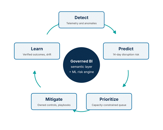
The contributions are: (1) an evaluation protocol that reports discrimination, calibration, and capacity-constrained performance side by side, including a prevalence-referenced Brier skill score; (2) a closed-loop BI and machine learning architecture (Figure 1) linking detection, prediction, prioritization, mitigation, and learning under NIST CSF 2.0 and the AI Risk Management Framework (National Institute of Standards and Technology [NIST], 2023, 2024); and (3) a transparent account of what a simulation can and cannot establish in this domain.

2. Related Work

2.1 Machine learning for cyber risk and incident forecasting

Surveys of data mining and machine learning for intrusion detection describe a large body of work on network, host, and malware detection (Buczak & Guven, 2016). Fewer studies forecast incidents at the organization level. Liu et al. (2015) predicted organizational breaches from externally observable indicators such as misconfiguration and malicious-activity signals, showing that enterprise-level forecasting is feasible with real data. The present study adopts a similar organization-level unit but uses a weekly enterprise panel and an explicit capacity constraint. Methodological critiques caution that security models often look better in development than in deployment because of sampling bias, label noise, temporal leakage, and lab-only evaluation (Arp et al., 2022; Sommer & Paxson, 2010); these pitfalls are discussed against our own design in Section 5.4.

2.2 Imbalance, calibration, and cost-sensitive decisions

Precision–recall curves are preferred when positives are uncommon (Saito & Rehmsmeier, 2015). Probability quality is commonly assessed with the Brier score (Brier, 1950); because the raw score depends on prevalence, it should be compared with a reference forecast that always predicts the base rate. Tree ensembles and reweighted models can produce distorted probabilities, which can be corrected with Platt scaling or isotonic regression (Niculescu-Mizil & Caruana, 2005; Platt, 1999; Zadrozny & Elkan, 2002). Reweighting or resampling classes also shifts a logistic model’s intercept, which can be corrected analytically (King & Zeng, 2001). Cost-sensitive learning shows that the optimal threshold depends on the costs of false positives and false negatives (Elkan, 2001).

2.3 Explainable AI in cybersecurity

Explainability surveys in cybersecurity emphasize that analysts need reasons, not just scores (Charmet et al., 2022; Rjoub et al., 2023; Yan et al., 2022). Permutation importance (Breiman, 2001) and Shapley-value attributions (Lundberg & Lee, 2017; Lundberg et al., 2020) are widely used, but both describe model behavior rather than causal effects, and permutation importance can be misleading when predictors are correlated (Strobl et al., 2008).

2.4 Governance frameworks

NIST CSF 2.0 adds a Govern function to the identify–protect–detect–respond–recover cycle (NIST, 2024); the AI RMF addresses mapping, measuring, and managing AI risk (NIST, 2023); zero-trust architecture removes implicit trust based on network location (Rose et al., 2020); and current incident-response guidance aligns response with CSF 2.0 (Nelson et al., 2025). Vulnerability prioritization can draw on the CISA Known Exploited Vulnerabilities (KEV) catalog (Cybersecurity and Infrastructure Security Agency [CISA], n.d.) and enterprise patch-management guidance (Souppaya & Scarfone, 2022), while supplier risk is addressed by NIST SP 800-161r1 (Boyens et al., 2022). Public companies must also disclose material cybersecurity incidents and risk-management processes (U.S. Securities and Exchange Commission [SEC], 2023). The gap addressed here is the absence of an evaluation design that ties these governance expectations to the statistical properties of the forecasts used to prioritize work.

3. Methods

3.1 Study design

This is a simulation study. A synthetic enterprise-week panel was generated so that analytical methods could be compared under known conditions; no real organizational records were used. Published 2025 industry reports informed the choice of feature domains and the direction of their associations with disruption, but no report supplied firm-level data, and generator parameters were not estimated from observational data. Because the outcome is generated from the predictors, which features matter and by how much is determined by the generator; the study therefore evaluates methods rather than real-world risk factors.

3.2 Synthetic panel

The panel contains 600 enterprise profiles observed weekly for 52 weeks (31,200 enterprise-weeks) across ten sectors: financial services, healthcare, manufacturing, retail, technology, professional services, transportation, energy, education, and government contracting (Table 1). Each row contains twenty predictors, a binary indicator of material disruption within the following fourteen days, downtime, and estimated financial loss. Only the disruption indicator is a prediction target; downtime and loss are used in scenario illustrations only. A late-year increase in threat pressure was included so that the test period differs from the training period, mimicking non-stationarity.

Supplementary Material S1 Reproducible replacement experiment: This supplement specifies the newly executed experiment used in the completed technical revision of manuscript 10974. It replaces the earlier draft's undocumented numerical illustration. No attempt is made to claim that the old performance values were reproduced. Every enterprise, sector effect, predictor, incident, downtime value, and financial loss is artificial. The associated code and exports are provided so that the revised numerical claims can be checked independently.

3.3 Predictors

Table 1. Synthetic panel design. All records and outcomes are synthetic. Published industry reports informed the choice of feature domains but did not supply firm-level data.

Design element

Specification

Unit of analysis

Enterprise-week snapshot

Population and period

600 simulated enterprise profiles × 52 weeks = 31,200 enterprise-weeks

Sectors (10)

Financial services, healthcare, manufacturing, retail, technology, professional services, transportation, energy, education, government contracting

Predictors

20 (Table 2)

Target

Material disruption within the following 14 days (binary)

Non-target outcomes

Downtime; estimated financial loss (scenario illustrations only)

Training set

Weeks 1–39; 23,400 enterprise-weeks

Test set

Weeks 40–52; 7,800 enterprise-weeks; 1,621 positive (20.8%)

Non-stationarity

Increased threat pressure in late-year weeks

Figure 1. Closed-loop business intelligence and machine learning framework. Telemetry is detected, converted to 14-day disruption forecasts, prioritized within review capacity, routed to owned controls and playbooks, and verified outcomes feed back into monitoring and retraining. The governed semantic layer supplies shared definitions to every stage. Conceptual design; not deployed in this study.

Table 2. Predictor dictionary. Note. Eighteen predictors are named in the original study materials; the authors must identify the remaining two. Descriptions are inferred from variable names and must be confirmed against the generator.

Domain

Variable

Description [AUTHOR INPUT: units and distribution for each]

Identity

failed_logins

Count of failed authentication attempts in the week.
Unit: authentication attempts/week. Distribution: Poisson(mean=12).

Identity

identity_risk

Composite identity-risk score.
Unit: dimensionless score, 0–1. Distribution: Beta(shapes=2,5).

Identity

impossible_travel

Count of geographically implausible sign-ins.
Unit: sign-ins/week. Distribution: Poisson(mean=0.6).

Identity

privilege_anomaly

Count of anomalous privilege changes.
Unit: privilege changes/week. Distribution: Poisson(mean=0.8).

Endpoint and email

malware_free_activity

Suspicious activity without a conventional malware indicator.
Unit: dimensionless score, 0–1. Distribution: Beta(shapes=1.5,6).

Endpoint and email

endpoint_alerts

Count of endpoint detection alerts.
Unit: alerts/week. Distribution: Poisson(mean=5).

Endpoint and email

email_phish_score

Phishing exposure score.
Unit: dimensionless score, 0–1. Distribution: Beta(shapes=2,6).

Cloud and vulnerability

cloud_misconfig

Count or score of cloud misconfigurations.
Unit: unresolved misconfigurations at the snapshot (count). Distribution: Poisson(mean=3).

Cloud and vulnerability

exposed_kev

Count of exposed CISA Known Exploited Vulnerabilities.
Unit: exposed vulnerabilities at the snapshot (count). Distribution: Poisson(mean=1).

Cloud and vulnerability

patch_latency_days

Days from patch availability to remediation.
Unit: days. Distribution: Gamma(shape=2,scale=8).

Cloud and vulnerability

external_surface

External attack-surface score.
Unit: dimensionless score, 0–1. Distribution: Beta(shapes=2,4).

Supplier and data

third_party_risk

Composite third-party risk score.
Unit: dimensionless score, 0–1. Distribution: Beta(shapes=2,3).

Supplier and data

vendor_dependency

Dependence on critical suppliers.
Unit: dimensionless score, 0–1. Distribution: Beta(shapes=2,2).

Supplier and data

data_egress_gb

Outbound data volume (GB).
Unit: gigabytes/week. Distribution: Lognormal(log-mean=2.5,log-SD=0.7).

Supplier and data

shadow_ai_risk

Ungoverned AI-use exposure score.
Unit: dimensionless score, 0–1. Distribution: Beta(shapes=1.5,6).

Business context

backup_health

Backup readiness score.
Unit: dimensionless score, 0–1; higher is better. Distribution: Beta(shapes=6,2).

Business context

business_criticality

Criticality of supported services.
Unit: ordinal integer, 1–5. Distribution: Discrete uniform {1,2,3,4,5}.

Business context

security_maturity

Security-program maturity score.
Unit: dimensionless score, 0–1; higher is better. Distribution: Beta(shapes=5,2).

Identity

mfa_coverage

Proportion of accounts protected by multi-factor authentication (MFA).
Unit: fraction, 0–1. Distribution: Beta(shapes=7,2).

Cloud and vulnerability

remote_access_exposure

Remote-access exposure score.
Unit: dimensionless score, 0–1. Distribution: Beta(shapes=2,5).

Table 3. Model specification. Note. Highlighted cells must be completed by the authors from the original analysis code.

Item

Logistic regression

Random forest

Gradient boosting

Implementation

scikit-learn 1.8.0
Logistic Regression

scikit-learn 1.8.0
Random Forest Classifier

scikit-learn 1.8.0
Gradient Boosting Classifier

Key hyperparameters

L2 regularization;
C = 1.0;
solver = lbfgs;
max_iter = 2,000.

n_estimators = 200;
max_depth = 10;
min_samples_leaf = 25;
max_features = sqrt;
bootstrap = True;
n_jobs = 1.

n_estimators = 150;
learning_rate = 0.05;
max_depth = 2;
min_samples_leaf = 25;
subsample = 1.0;
loss = log_loss.

Tuning procedure

Fixed settings; no search or cross-validation.

Fixed settings; no search or cross-validation.

Fixed settings; no search or cross-validation.

Class weighting

Yes. class weight = balanced.

Yes. class_weight = balanced

Yes. Balanced weights supplied through sample_weight.

Feature scaling

StandardScaler fitted on training data only.

Not required; no scaling applied.

Not required; no scaling applied.

Threshold (≈15% alerts)

Weekly top 90/600.
Median cutoff 0.7000; range 0.6844–0.7136.

Weekly top 90/600.
Median cutoff 0.5955; range 0.5846–0.6124.

Weekly top 90/600.
Median cutoff 0.6548; range 0.6307–0.6757.

Table 4. Temporal test-set performance (n = 7,800; 1,621 positives). Note. BSS = Brier skill score relative to a constant forecast equal to the test prevalence (0.208); negative values indicate worse-than-reference probabilities. ROC-AUC intervals use the Hanley–McNeil approximation; precision and recall intervals are Wilson intervals. Each model flags 1,152 enterprise-weeks (14.8%). F1 = 0.391, 0.366, and 0.367. The no-skill row assumes random selection of the same alert volume.

Model

ROC-AUC (95% CI)

PR-AUC

Brier

BSS

Precision (95% CI)

Recall (95% CI)

Logistic regression

0.701 (0.686–0.716)

0.407

0.206

−0.251

47.0% (44.2–49.9)

33.4% (31.2–35.8)

Random forest

0.694 (0.679–0.709)

0.395

0.189

−0.148

44.1% (41.3–47.0)

31.3% (29.1–33.6)

Gradient boosting

0.693 (0.678–0.708)

0.396

0.150

0.089

44.2% (41.3–47.1)

31.4% (29.2–33.7)

No-skill reference

0.500

0.208

0.165

0.000

20.8%

14.8%


Table 5. Assumption-driven scenario outputs (illustrative, not estimates). Note. Control indices must not be added or multiplied to infer combined effects. Mean predicted risk inherits the calibration error reported in Table 4.


Scenario

Output

Interpretation

Third-party exposure quintiles

Modeled disruption rate ≈15% (Q1) to ≈29% (Q5)

Gradient built into generator

MFA and conditional access

Residual-risk index 100 → ≈57

Assumed control effect

Accelerated KEV patching

100 → ≈68

Assumed control effect

Network segmentation

100 → ≈72

Assumed control effect

Endpoint and identity analytics

100 → ≈54

Assumed control effect

Third-party access review

100 → ≈65

Assumed control effect

Immutable backups

100 → ≈61

Assumed control effect

Cost–benefit curve

Net value peaks at ≈14.9% alert rate

Depends on assumed costs

Stress: baseline / phishing / zero-day / supplier outage / shadow-AI / combined

Mean predicted risk ≈44 / 54 / 60 / 58 / 52 / 76%; continuity index 1.00 / 0.86 / 0.78 / 0.73 / 0.88 / 0.61

Assumed shock multipliers

Drift monitoring (12 months)

PSI exceeds 0.20 review reference, then declines

Illustrative monitoring trace

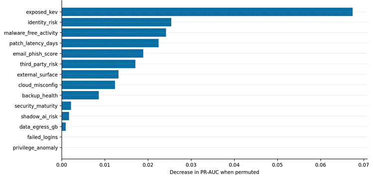
Twenty predictors spanned identity, endpoint and email, cloud and vulnerability, supplier and data, and business-context domains (Table 2). All predictors were constructed from information available at or before the snapshot week. Variable names in Figure 3 correspond to the identifiers in Table 2.

3.4 Temporal partition and leakage control

Weeks 1–39 (23,400 observations) were used for training and weeks 40–52 (7,800 observations) for testing, so that each model was evaluated on later observations than it was trained on. Because the outcome horizon (fourteen days) exceeds the snapshot interval (one week), labels for the final training weeks overlap the test period. In the replacement simulation, all three models were refitted using weeks 1–37 (22,200 observations), with weeks 38–39 embargoed and weeks 40–52 reserved for testing (7,800 observations). The final training outcome window ended at week 39, preventing fourteen-day labels from extending into the test forecast period. The twenty predictors, prespecified hyper parameters, weighting schemes, and random seed (20261028) were retained; preprocessing was fitted exclusively on training data. Compared with training on weeks 1–39, the maximum absolute change was 0.000864 in ROC-AUC and 0.002362 in average precision. Logistic regression retained the highest discrimination on both metrics, while random forest and gradient boosting exchanged average-precision ranks.

The same 600 enterprises appear in both partitions, so the design tests temporal generalization within known enterprises, not transfer to new organizations.

3.5 Models

Three model families were compared: L2-regularized logistic regression as a transparent baseline, random forest (Breiman, 2001) to capture nonlinear interactions, and gradient boosting (Friedman, 2001). All models used class weighting to address imbalance. Hyperparameters were selected using training data only (Table 3). The operating threshold for each model was chosen to produce an alert volume of approximately 15% of enterprise-weeks, representing an assumed review capacity; for logistic regression this corresponded to a predicted probability of 0.644.

3.6 Evaluation

Discrimination was measured by ROC-AUC and PR-AUC. In the replacement analysis, PR-AUC was defined as non-interpolated average precision (AP) and computed using sklearn. metrics. average_precision_score(y_true, y_score) in scikit-learn 1.8.0. AP summarizes precision across score thresholds, weighting each precision value by the corresponding increase in recall (scikit-learn developers, n.d.):

AP = k = 1K(Rk - Rk-1)Pk

Here, Pₖ and Rₖ denote precision and recall at threshold k, K is the number of threshold steps, and R₀ = 0 when recall is ordered from zero upward. This calculation uses recall increments without trapezoidal interpolation.

The calculation used all 7,800 held-out enterprise-weeks from weeks 40–52, with fourteen-day disruption coded as the positive class (y = 1). Scores were each model’s continuous positive-class probabilities from predict_proba(X_test) [: 1]; no evaluation sample weights were applied. AP assessed ranking across thresholds, while precision and recall under the 15% weekly review-capacity policy were evaluated separately.

Because individual test-set predictions were not available for this revision, 95% confidence intervals for ROC-AUC were approximated with the Hanley–McNeil method (Hanley & McNeil, 1982); a paired DeLong test (DeLong et al., 1988) should replace this once predictions are re-generated For the replacement analysis, paired DeLong tests comparing ROC-AUC yielded \(p=8.61\times10^{-7}\) for logistic regression versus random forest, \(p=8.97\times10^{-6}\) for logistic regression versus gradient boosting, and \(p=0.392\) for random forest versus gradient boosting. PR-AUC, defined as average precision, and its 95% bootstrap confidence interval were 0.5620 (0.5172–0.6059), 0.5402 (0.4934–0.5863), and 0.5423 (0.4982–0.5885), respectively. Intervals used 500 paired enterprise-cluster resamples, retaining each enterprise’s thirteen-week test trajectory with fitted models held fixed. DeLong p-values are descriptive because their conventional calculation ignores within-enterprise dependence; clustered bootstrap intervals provide the primary uncertainty assessment. Probability quality was measured by the Brier score and the Brier skill score, BSS = 1 − BS/BSref, where BSref = p(1 − p) is the score of a constant forecast equal to the test prevalence p; BSS > 0 indicates improvement over that reference. At the operating threshold we report precision, recall, and F1 with Wilson 95% confidence intervals (Wilson, 1927), and the lift of precision over prevalence.

3.7 Explanations

Global importance was measured by permutation importance on the test set as the decrease in PR-AUC after randomly permuting one predictor For the replacement analysis, permutation importance was calculated for the fitted logistic regression model using 20 repeats per predictor and numpy. random.default_rng(20261228). For each repeat, one predictor’s complete thirteen-week trajectory was randomly reassigned among the 600 enterprises in the test set. Outcomes, other predictors, and the fitted model remained unchanged; no retraining was performed. Importance was calculated as:

Ij = 120r = 120(APoriginal - APj,rpermuted)

Here, Iⱼ is the importance of predictor j, r indexes the twenty permutation repeats, and AP denotes non-interpolated average precision. Each term is the original test-set AP minus the AP obtained after permuting predictor j in repeat r.

Larger positive values indicate greater deterioration in average precision after permutation. Figure error bars represent the sample standard deviation across the twenty repeats (ddof = 1), not confidence intervals. These importance values describe model dependence and do not establish causal effects.

A local explanation of a single high-risk enterprise-week was produced as signed contributions on the log-odds scale In the replacement analysis, local explanations used an exact decomposition of logistic-regression log odds:


φj = βjxj - μjsj

logit(p) = β0 + j = 120φj

Here, φⱼ is predictor j’s signed contribution, xⱼ is its observed value, and μⱼ and sⱼ are its mean and standard deviation estimated exclusively from training data. The coefficient β̂ⱼ is the fitted logistic-regression coefficient for the standardized predictor, and β̂₀ is the fitted intercept.

The reference point was the vector of training-set feature means, corresponding to zero after standardization; baseline log odds equaled the fitted intercept. Adding all twenty contributions to this intercept exactly reconstructed the model’s predicted log odds.

Positive contributions increased predicted log odds relative to this reference, while negative contributions decreased them. These attributions describe model behavior, not causal effects.

Both describe model behavior, not intervention effects.

3.8 Decision scenarios

Several assumption-driven scenarios illustrate how forecasts could be used in planning: a third-party exposure gradient, six control scenarios expressed on a residual-risk index (baseline = 100), a cost–benefit curve across alert rates, five stress scenarios, and a population stability index (PSI) monitoring trace. The control reductions and stress effects were specified by the authors, not estimated. Scenario assumptions for the replacement analysis.

All values below are explicit assumptions used in the executed replacement simulation. Control indices, prevention probability, costs, and continuity indices were stipulated; they are not estimated treatment effects or observed enterprise benefits. Supplementary table S2A, S2B, S2C.


V = 0.10 × 20,000 × Ncovered - 250 × Nreviews

V is assumed expected net value in USD relative to no review. A covered incident has at least one alert for the same enterprise one or two weeks earlier. Each incident is counted once even when alert windows overlap. Uncovered incidents retain the full assumed loss; covered incidents retain 90% in expectation. The fixed USD 20,000 scenario loss is distinct from the generator’s variable synthetic loss field.

The continuity indices are separately stipulated assumptions: baseline 1.00, phishing 0.86, vulnerability pressure 0.78, supplier outage 0.73, shadow AI 0.88, and combined 0.61. They are not derived from predicted probabilities or from observed business continuity outcomes.

The historical “Zero-day” scenario label denotes illustrative vulnerability pressure represented by two additional exposed known exploited vulnerabilities and longer patch latency. It is not a validated simulation of an unknown vulnerability. Predicted probabilities remain raw model outputs and inherit the calibration limitations of the replacement analysis.

3.8.1 Alert and incident counting rules

For each test forecast week (40–52), enterprises are ranked by descending raw logistic score; ascending enterprise ID resolves ties. The review count is floor (capacity × 600). Utility covers underlying incident weeks 41–54. An incident is covered only by an available test-period alert from its preceding one- or two-week window; the union of those windows prevents duplicate counting. Expected prevention benefits are calculated, not simulated as additional incident outcomes. The capacity maximizing this utility is selected with hindsight and is not a prospectively validated operating policy. Supplementary table S2D.

3.8.2 Implementation record

All numeric assumptions are transcribed from scenario_assumptions. json and the scenario analysis function in analysis.py. The fixed models belong to the executed replacement experiment (model random seed 20261028). Scenario transformations are deterministic and introduce no additional random draws. These specifications do not reconstruct the original manuscript’s undocumented scenario calculations.

Scenario outputs are reported in Table 5 and are not used to support empirical claims.

3.9 BI architecture

The proposed architecture (Figure 1) ingests identity, endpoint, email, cloud, vulnerability, and supplier telemetry through a streaming layer into a lakehouse and feature store. A governed semantic model defines shared enterprise, asset, time, threat, identity, and vendor dimensions, so that executive and security operations center (SOC) dashboards use the same measure definitions. Each forecast record stores the snapshot time, horizon, model version, explanation, reviewer, action, and verified outcome. This architecture is a design proposal; it was not deployed in this study.

4. Results

4.1 Test set

The test set contained 7,800 enterprise-weeks, of which 1,621 were positive (prevalence 20.8%). The Brier reference score for this prevalence is 0.165, and the no-skill PR-AUC is 0.208.

4.2 Discrimination

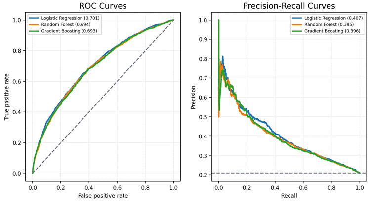
Discrimination was modest and similar across models (Table 4; Figure 2). Logistic regression achieved ROC-AUC 0.701 (95% CI 0.686–0.716) and PR-AUC 0.407, random forest 0.694 (0.679–0.709) and 0.395, and gradient boosting 0.693 (0.678–0.708) and 0.396. The confidence intervals overlap substantially, so the data do not show that any model ranks better than the others. PR-AUC values were approximately 1.9–2.0 times the no-skill level.

4.3 Probability quality

Calibration ordered the models differently. Brier scores were 0.206 (logistic regression), 0.189 (random forest), and 0.150 (gradient boosting), giving Brier skill scores of −0.251, −0.148, and 0.089. Thus the logistic and random-forest probabilities were less accurate than simply predicting the base rate for every enterprise-week, and gradient boosting improved on the base rate only slightly. Consistent with this, the mean predicted risk of the logistic model was 43.8%, about twice the observed 20.8%. This overestimation is the expected consequence of class weighting, which trains the model as if positives and negatives were balanced. Answering RQ1, the model with the best ranking (logistic regression) had the worst probability quality.

4.4 Capacity-constrained operating point

At the logistic threshold of 0.644, the model produced 542 true positives, 610 false positives, 1,079 false negatives, and 5,569 true negatives. It flagged 1,152 enterprise-weeks (14.8%) with precision 47.0% (95% CI 44.2–49.9%), recall 33.4% (31.2–35.8%), and F1 0.391. Precision was 2.3 times the base rate, so the queue was considerably richer in disruption windows than random selection. At the same alert volume, random forest identified 508 positives (precision 44.1%, recall 31.3%) and gradient boosting 509 (44.2%, 31.4%). An approximate unpaired comparison of logistic and random-forest precision did not show a significant difference (z = 1.42, p = .16). Answering RQ2, a capacity-feasible queue concentrated risk but missed about two-thirds of positive windows.

4.5 Global and local explanations

Permutation importance for the logistic model was highest

Figure 2. ROC and precision–recall curves on the temporal test set (weeks 40–52). Legend values are ROC-AUC (left) and PR-AUC (right). Dashed lines show chance (left) and prevalence, 0.208 (right). Synthetic data.

Figure 3. Permutation importance of predictors in the logistic regression model. Bars show the decrease in test-set PR-AUC when each predictor is permuted. Variable names are defined in Table 2. Fourteen of twenty predictors are displayed All twenty predictors are displayed, with variable names defined in Table 2. Importance reflects the data-generating process and model dependence, not causal control benefit.

for exposed KEVs (decrease in PR-AUC ≈ 0.067), followed by identity risk, malware-free activity, patch latency, phishing score, third-party risk, external attack surface, cloud misconfiguration, and backup health (each 0.008–0.025; Figure 3). Security maturity, shadow-AI risk, and data egress contributed little, and failed logins and privilege anomalies contributed approximately zero. Because the outcome was generated by the authors, this ranking recovers the strength of each predictor in the generator; it is a check that the explanation method works, not evidence about real-world risk factors. The near-zero importance of failed logins and privilege anomalies may also reflect overlap with the composite identity-risk score (Strobl et al., 2008). In the local example, exposed vulnerabilities and patch latency were the largest positive contributors, with backup health, phishing, and malware-free activity also raising the score, while data egress and cloud misconfiguration lowered it for that enterprise-week.

4.6 Scenario illustrations

Table 5 summarizes the assumption-driven scenario outputs. Modeled disruption rates rose from about 15% to 29% across third-party exposure quintiles; the control scenarios reduced the residual-risk index to between 54 and 72; net value in the cost illustration peaked near a 14.9% alert rate; and a combined shock raised mean predicted risk to about 76% and lowered the continuity index to 0.61. Because these quantities follow directly from the assumptions in Section 3.8, they show how the framework would present such analyses and should not be read as estimates of control effectiveness or economic benefit.

5. Discussion

5.1 Principal findings

The simulation shows three points. First, the three model families ranked enterprise-weeks almost equally well, so added model complexity did not improve discrimination when relationships were largely additive. Second, ranking and probability quality diverged sharply: the best-ranking model produced probabilities worse than a base-rate forecast. Any expected-loss figure, risk tier, or board metric computed from such probabilities would overstate risk roughly twofold. Third, at a realistic review capacity, the best queue was 2.3 times richer in disruption windows than random review yet missed two-thirds of them, so absence of an alert cannot be taken as assurance.

5.2 Comparison with prior work

The calibration result agrees with evidence that reweighting and many ensemble methods distort probabilities (King & Zeng, 2001; Niculescu-Mizil & Caruana, 2005). The practical lesson is that class weighting is acceptable for ranking but should be followed by recalibration—prior correction of the intercept, Platt scaling, or isotonic regression on a held-out calibration period—before probabilities are reported. The modest ROC-AUC of about 0.70 is lower than reported for organization-level breach forecasting from real external signals (Liu et al., 2015); differences in outcome definition, horizon, and data make direct comparison inappropriate, but the result shows that the simulated task was not made artificially easy. The near-identical performance of linear and ensemble models echoes concerns that complex models are often adopted without demonstrated gains in security settings (Arp et al., 2022).

5.3 Implications for practice

Answering RQ3, the framework suggests four practices. (1) Report ROC-AUC, PR-AUC, Brier skill score, and capacity-constrained precision and recall together, and choose the model according to the decision it supports: a ranking model for queue ordering and a calibrated model for expected-loss estimation. (2) Set thresholds from review capacity and the relative cost of missed and unnecessary investigations (Elkan, 2001) rather than at 0.50. (3) Treat explanations as pointers to evidence: a high contribution from exposed KEVs should lead an analyst to the affected asset, its exposure date, and remediation status (CISA, n.d.; Souppaya & Scarfone, 2022), not directly to an action. (4) Use the BI semantic layer to keep the unit of every measure explicit—enterprise-week, asset, case, or incident—so that executive and SOC dashboards cannot report incompatible counts as comparable.

Governance requirements follow from the same logic. High-impact actions such as account restriction or supplier access revocation should require documented human approval; each forecast record should retain model version, evidence, reviewer, action, and verified outcome; and monitoring should track input drift (e.g., PSI), PR-AUC, and calibration separately, because a change in any one can reflect new controls, collection failures, delayed labels, or attacker behavior rather than model decay. Behavioral telemetry used for identity analytics should be collected proportionately, with role-based access and defined retention, consistent with the NIST AI RMF (NIST, 2023). Unreviewed cases should not be treated as negatives when retraining, because only investigated cases acquire verified labels.

5.4 Limitations

The main limitation is that all data are synthetic. Feature importance, the third-party gradient, control reductions, and stress effects reflect the generator and scenario assumptions; they cannot identify real risk factors or causal control benefits. Second, the analysis is subject to the pitfalls identified by Arp et al. (2022): evaluation is lab-only, enterprises are shared between training and test periods, and the fourteen-day label horizon may overlap the train–test boundary (Section 3.4). Third, confidence intervals for ROC-AUC were approximated without access to individual predictions, and no paired test or PR-AUC interval could be computed. Fourth, recalibrated models were not fitted, so the extent to which recalibration would close the gap between ranking and probability quality remains to be shown. Fifth, enterprise-week positives are forecast windows, not unique incidents; neighboring windows can refer to the same simulated episode, which inflates the apparent number of events. Finally, the BI architecture and dashboards were designed but not deployed, and no user study assessed whether analysts interpret explanations correctly.

5.5 Future research

Priority extensions are: (a) validation on longitudinal enterprise incident data, holding out whole organizations as well as later time periods; (b) recalibration and comparison of calibrated expected-loss estimates with realized losses; (c) quasi-experimental or randomized evaluation of control interventions to replace assumed control effects; (d) graph-based modeling of attack paths and supplier dependencies; (e) privacy-preserving or federated learning across organizations; and (f) user studies of explanation-assisted triage.

6. Conclusion

In a controlled simulation of 31,200 enterprise-weeks, logistic regression, random forest, and gradient boosting ranked disruption risk about equally well, but the best-ranking model produced the least reliable probabilities, and a capacity-feasible queue captured only one-third of disruption windows. Cyber-risk forecasts should therefore be evaluated on discrimination, calibration, and capacity together, recalibrated before use in financial reporting, and linked through a governed BI layer to evidence and accountable owners. The framework is ready for empirical testing; its value for real enterprises remains to be demonstrated with organizational data.

Author contributions

M.H. Conceptualization; Methodology; Formal analysis; Writing – original draft. M.R.H. Investigation; Validation; Writing – review and editing. K.R.H.S. Methodology; Project administration; Writing – review and editing. M.A.R. Software; Data curation; Validation; Visualization; Writing – review and editing. M.F.A.B. Investigation; Validation; Writing – review and editing.

Competing financial interests

The authors MH et al., have no conflict of interest.

Generative AI statement

The authors declare that Gen AI was used in the creation of this manuscript. Generative AI was used in the preparation of this manuscript in a limited and strictly controlled manner. Specifically, it assisted during the initial organization of thematic sections and helped identify general areas of literature for further manual exploration. All writing, analysis, interpretation, and synthesis of content were performed by the authors. All references in the current version have been manually reviewed and verified. The final manuscript has been completely revised to ensure originality, accuracy, and integrity, fully aligning with COPE policies on the responsible use of generative AI.

Data availability statement

The data supporting the findings of this study are derived from the synthetic dataset, underlying weekly incident records, predictor dictionary, and data generator for the replacement analysis are included in the accompanying 10974_Reproducibility_Package.zip. The panel contains 31,200 enterprise-week observations from 600 artificial enterprises over 52 forecast weeks. The generator uses random seed 20261028. No real organizational or personal records are included. The generated CSV data are supplied under CC0 1.0 Universal, with data-file checksums included in the package. Public repository deposition has not yet been completed, and a repository DOI has not been assigned

The accompanying reproducibility package contains the Python code for data generation, model training, the embargo sensitivity comparison, statistical evaluation, bootstrap intervals, model explanations, scenario calculations, and figure generation for the replacement analysis. The code is supplied under the MIT License. Software version requirements, random seeds, execution instructions, and saved results are provided to support independent reproduction and review. These files document the replacement experiment and do not establish the provenance of the original manuscript’s numerical results. A public repository DOI for the code has not yet been assigned.

References


Arp, D., Quiring, E., Pendlebury, F., Warnecke, A., Pierazzi, F., Wressnegger, C., Cavallaro, L., & Rieck, K. (2022). Dos and don’ts of machine learning in computer security. In Proceedings of the 31st USENIX Security Symposium (pp. 3971–3988). USENIX Association.

Boyens, J., Smith, A., Bartol, N., Winkler, K., Holbrook, A., & Fallon, M. (2022). Cybersecurity supply chain risk management practices for systems and organizations (NIST Special Publication 800-161r1). National Institute of Standards and Technology. https://doi.org/10.6028/NIST.SP.800-161r1

Breiman, L. (2001). Random forests. Machine Learning, 45(1), 5–32. https://doi.org/10.1023/A:1010933404324

Brier, G. W. (1950). Verification of forecasts expressed in terms of probability. Monthly Weather Review, 78(1), 1–3. https://doi.org/10.1175/1520-0493(1950)078<0001:VOFEIT>2.0.CO;2

Buczak, A. L., & Guven, E. (2016). A survey of data mining and machine learning methods for cyber security intrusion detection. IEEE Communications Surveys & Tutorials, 18(2), 1153–1176. https://doi.org/10.1109/COMST.2015.2494502

Charmet, F., Tanuwidjaja, H. C., Ayoubi, S., Gimenez, P.-F., Han, Y., Jmila, H., Blanc, G., Takahashi, T., & Zhang, Z. (2022). Explainable artificial intelligence for cybersecurity: A literature survey. Annals of Telecommunications, 77, 789–812. https://doi.org/10.1007/s12243-022-00926-7

Cybersecurity and Infrastructure Security Agency. (n.d.). Known exploited vulnerabilities catalog. Retrieved, from https://www.cisa.gov/known-exploited-vulnerabilities-catalog

DeLong, E. R., DeLong, D. M., & Clarke-Pearson, D. L. (1988). Comparing the areas under two or more correlated receiver operating characteristic curves: A nonparametric approach. Biometrics, 44(3), 837–845. https://doi.org/10.2307/2531595

Elkan, C. (2001). The foundations of cost-sensitive learning. In Proceedings of the 17th International Joint Conference on Artificial Intelligence (pp. 973–978).

Few, S. (2013). Information dashboard design: Displaying data for at-a-glance monitoring (2nd ed.). Analytics Press.

Friedman, J. H. (2001). Greedy function approximation: A gradient boosting machine. The Annals of Statistics, 29(5), 1189–1232. https://doi.org/10.1214/aos/1013203451

Hanley, J. A., & McNeil, B. J. (1982). The meaning and use of the area under a receiver operating characteristic (ROC) curve. Radiology, 143(1), 29–36. https://doi.org/10.1148/radiology.143.1.7063747

IBM. (2025). Cost of a data breach report 2025. IBM Security. https://www.ibm.com/reports/data-breach

Kimball, R., & Ross, M. (2013). The data warehouse toolkit: The definitive guide to dimensional modeling (3rd ed.). Wiley.

King, G., & Zeng, L. (2001). Logistic regression in rare events data. Political Analysis, 9(2), 137–163. https://doi.org/10.1093/oxfordjournals.pan.a004868

Liu, Y., Sarabi, A., Zhang, J., Naghizadeh, P., Karir, M., Bailey, M., & Liu, M. (2015). Cloudy with a chance of breach: Forecasting cyber security incidents. In Proceedings of the 24th USENIX Security Symposium (pp. 1009–1024). USENIX Association.

Lundberg, S. M., Erion, G., Chen, H., DeGrave, A., Prutkin, J. M., Nair, B., Katz, R., Himmelfarb, J., Bansal, N., & Lee, S.-I. (2020). From local explanations to global understanding with explainable AI for trees. Nature Machine Intelligence, 2, 56–67. https://doi.org/10.1038/s42256-019-0138-9

Lundberg, S. M., & Lee, S.-I. (2017). A unified approach to interpreting model predictions. In Advances in Neural Information Processing Systems 30 (pp. 4765–4774).

National Institute of Standards and Technology. (2023). Artificial intelligence risk management framework (AI RMF 1.0) (NIST AI 100-1). https://doi.org/10.6028/NIST.AI.100-1

National Institute of Standards and Technology. (2024). The NIST cybersecurity framework (CSF) 2.0 (NIST CSWP 29). https://doi.org/10.6028/NIST.CSWP.29

Nelson, A., Rekhi, S., Souppaya, M., & Scarfone, K. (2025). Incident response recommendations and considerations for cybersecurity risk management: A CSF 2.0 community profile (NIST Special Publication 800-61r3). National Institute of Standards and Technology. https://doi.org/10.6028/NIST.SP.800-61r3

Niculescu-Mizil, A., & Caruana, R. (2005). Predicting good probabilities with supervised learning. In Proceedings of the 22nd International Conference on Machine Learning (pp. 625–632). https://doi.org/10.1145/1102351.1102430

Platt, J. (1999). Probabilistic outputs for support vector machines and comparisons to regularized likelihood methods. In A. Smola, P. Bartlett, B. Schölkopf, & D. Schuurmans (Eds.), Advances in large margin classifiers (pp. 61–74). MIT Press.

Rjoub, G., Bentahar, J., Wahab, O. A., Mizouni, R., Song, A., Cohen, R., Otrok, H., & Mourad, A. (2023). A survey on explainable artificial intelligence for cybersecurity. IEEE Transactions on Network and Service Management, 20(4), 5115–5140. https://doi.org/10.1109/TNSM.2023.3282740

Rose, S., Borchert, O., Mitchell, S., & Connelly, S. (2020). Zero trust architecture (NIST Special Publication 800-207). National Institute of Standards and Technology. https://doi.org/10.6028/NIST.SP.800-207

Saito, T., & Rehmsmeier, M. (2015). The precision-recall plot is more informative than the ROC plot when evaluating binary classifiers on imbalanced datasets. PLOS ONE, 10(3), e0118432. https://doi.org/10.1371/journal.pone.0118432

Sommer, R., & Paxson, V. (2010). Outside the closed world: On using machine learning for network intrusion detection. In 2010 IEEE Symposium on Security and Privacy (pp. 305–316). IEEE. https://doi.org/10.1109/SP.2010.25

Souppaya, M., & Scarfone, K. (2022). Guide to enterprise patch management planning: Preventive maintenance for technology (NIST Special Publication 800-40r4). National Institute of Standards and Technology. https://doi.org/10.6028/NIST.SP.800-40r4

Strobl, C., Boulesteix, A.-L., Kneib, T., Augustin, T., & Zeileis, A. (2008). Conditional variable importance for random forests. BMC Bioinformatics, 9, 307. https://doi.org/10.1186/1471-2105-9-307

U.S. Securities and Exchange Commission. (2023). Cybersecurity risk management, strategy, governance, and incident disclosure (Release No. 33-11216). https://www.sec.gov/rules/final/2023/33-11216.pdf

Verizon. (2025). 2025 data breach investigations report. Verizon Business. https://www.verizon.com/business/resources/reports/dbir/

Wilson, E. B. (1927). Probable inference, the law of succession, and statistical inference. Journal of the American Statistical Association, 22(158), 209–212. https://doi.org/10.1080/01621459.1927.10502953

Yan, F., Wen, S., Nepal, S., Paris, C., & Xiang, Y. (2022). Explainable machine learning in cybersecurity: A survey. International Journal of Intelligent Systems, 37(12), 12305–12334. https://doi.org/10.1002/int.23088

Zadrozny, B., & Elkan, C. (2002). Transforming classifier scores into accurate multiclass probability estimates. In Proceedings of the 8th ACM SIGKDD International Conference on Knowledge Discovery and Data Mining (pp. 694–699). https://doi.org/10.1145/775047.775151


Article metrics
View details
0
Downloads
0
Citations
304
Views
📖 Cite article

View Dimensions


View Plumx


View Altmetric


0
Save
0
Citation
304
View
0
Share