Journal of Ai ML DL

1.Introduction

Healthcare supply chains have always been complex, but the past decade has made one thing unmistakably clear: optimizing for efficiency alone is not enough. Across the United States and beyond, disparities in access to essential medical resources — pharmaceuticals, surgical supplies, diagnostic equipment — do not distribute randomly across populations. They cluster, predictably and persistently, along lines of income, race, geography, and education. These are not incidental patterns. They are the structural fingerprints of Social Determinants of Health (SDOH), and their consequences reach far beyond clinical settings into the very logistics systems that are supposed to serve everyone equitably (Kino et al., 2021).

Artificial intelligence has, in recent years, entered healthcare supply chain management with considerable enthusiasm. Demand forecasting, inventory control, delivery optimization — these are problems that machine learning handles well, and the literature reflects that promise (Periáñez et al., 2024). What it reflects less clearly is whether the systems being built actually serve all populations fairly, or whether they replicate — and in some cases amplify — the inequities already baked into the data they learn from. That concern is not hypothetical. Chen et al. (2023) documented how algorithmic systems trained on historically biased healthcare data can produce decision outputs that systematically disadvantage minority and low-income groups, even when no explicit discriminatory variable is included in the model. The bias is structural, and it travels invisibly through the pipeline.

SDOH variables — income level, racial and ethnic composition, educational attainment, neighborhood-level environmental risk — are established predictors of healthcare demand patterns. Communities with lower socioeconomic status tend to have higher rates of preventable illness, greater reliance on emergency care, and reduced access to primary and specialist services (Braveman & Gottlieb, 2014; Vyas et al., 2020). Despite this, the overwhelming majority of AI-based supply chain models treat demand as a purely clinical or operational signal. SDOH data, when collected at all, typically flows into epidemiological research rather than into the allocation algorithms that determine who receives resources, when, and in what quantity. The operational and the equitable remain, for now, largely separate conversations.

This separation matters because supply chain allocation is not a neutral act. From a systems perspective, every resource allocation decision made under conditions of structural inequity is a policy decision — whether or not it is recognized as one. If an AI model consistently predicts lower demand in a historically underserved ZIP code because that community has historically received fewer resources, the model will, left uncorrected, continue to justify underprovision. The feedback loop is self-reinforcing, and it is invisible to efficiency metrics (Obermeyer et al., 2019; Rajkomar et al., 2018).

Addressing this requires more than adding SDOH variables as features in a conventional predictive model. Statistical associations between SDOH and demand, while informative, do not distinguish between legitimate variation in clinical need and the structural suppression of that need by prior inequitable allocation. Causal inference offers a more principled approach. By modeling the structural pathways through which SDOH affects both demand and access — and by explicitly identifying which of those pathways represent allocable bias — causal frameworks allow researchers to intervene in the decision-making process in a targeted, justified way (Makhlouf et al., 2020; Pearl, 2009; Kusner et al., 2017).

Geospatial complexity adds a further dimension. Regional variation in healthcare demand is not simply a function of population size; it reflects proximity to facilities, transportation infrastructure, environmental hazards, and mobility constraints that cluster spatially in ways that conventional tabular modeling cannot adequately capture (Shang et al., 2024).

This paper attempts to bridge these gaps. It presents a fairness-aware AI framework that integrates SDOH data, causal structural modeling, geospatial machine learning, and multi-objective optimization into a unified healthcare supply chain decision system. Three models are compared — a conventional ML baseline, an SDOH-augmented model, and the proposed fairness-constrained model — across predictive, operational, and equity metrics. The central argument is not that efficiency and fairness must trade off against each other, but that, with the right structural design, they can reinforce each other. Whether that argument holds empirically, and under what conditions, is what this study sets out to examine (Liu et al., 2025; Banja et al., 2023).

2.Methodology

2.1 Framework Overview

The methodological approach taken here is deliberately integrative. Rather than treating fairness as a post-hoc correction — a layer applied after a model has already been trained — this framework builds fairness constraints into each stage of the pipeline, from data integration through causal modeling, geospatial prediction, and resource optimization. The architecture follows four sequential but interconnected layers: (i) multi-source data integration and preprocessing, (ii) Structural Causal Model (SCM) construction for bias identification, (iii) geospatial machine learning for spatially-aware demand forecasting, and (iv) fairness-constrained multi-objective optimization for resource allocation. Each layer informs the next, and fairness considerations propagate forward across all of them (Chen et al., 2023).

2.2 Data Integration and Preprocessing

Five primary data sources were integrated for this study (Table 1). Healthcare utilization data — including weekly hospital admissions, ICU occupancy rates, and disease incidence by county — were drawn from the Centers for Disease Control and Prevention (CDC) and state health agency repositories covering 2020–2024. Supply chain logistics data, comprising facility-level inventory levels, transportation cost per delivery, and delivery time in hours, were obtained from hospital systems supplemented with synthetically generated records where real supply chain records were restricted; the synthetic component was generated using distributional parameters derived from published healthcare logistics benchmarks and validated against the non-synthetic subset. SDOH data at census tract and county levels — income, race and ethnicity, educational attainment, and employment status — were sourced from the U.S. Census Bureau's American Community Survey (2019–2023). Geographic and adjacency data were obtained from the Census TIGER/Line shapefiles. Environmental health risk indicators, including particulate matter (PM2.5), proximity-to-hazard indices, and Environmental Justice (EJ) screening scores, came from the EPA's EJSCREEN database (2019–2024) (Kino et al., 2021).

All datasets were aligned to a common weekly temporal granularity. Spatial harmonization was performed using geographic identifiers (FIPS codes, ZIP codes) through GIS spatial join operations, enabling integration of healthcare, SDOH, environmental, and mobility data at consistent spatial units. A composite Vulnerability Index (VI) was constructed for each geographic unit as a weighted linear combination of standardized income deprivation, racial minority proportion, educational disadvantage score, and environmental risk index — weights derived from principal component analysis of these four domains, following the methodological approach used in the Social Vulnerability Index (Flanagan et al., 2011). An Accessibility Index was calculated using straight-line and road-network distance to the nearest primary care facility and specialist facility, weighted by provider density per 10,000 population from HRSA Area Health Resources Files. Missing data were addressed using multiple imputation by chained equations (MICE), with five imputation iterations; imputed values were evaluated for plausibility against observed marginal distributions prior to inclusion.

2.3 Structural Causal Model for Bias Identification

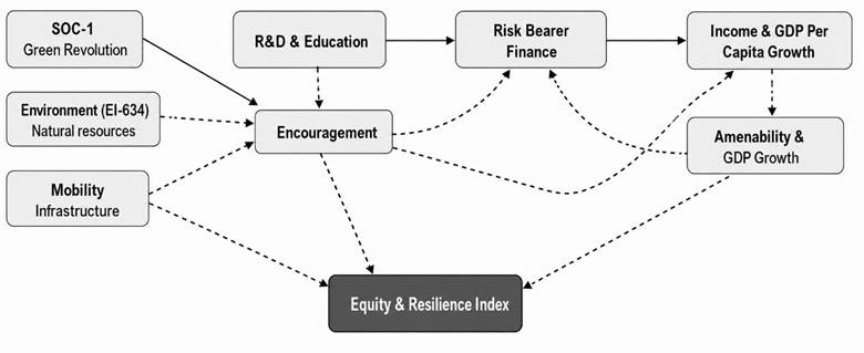
The causal modeling component addresses a problem that feature engineering alone cannot resolve: distinguishing structural suppression of healthcare demand from legitimate variation in clinical need. A Structural Causal Model (SCM) was formulated following the framework of Pearl (2009) and Hernán and Robins (2020). The causal graph specifies the following directed relationships:

SDOH variables (income, race, education, employment) → Healthcare demand
Environmental determinants (PM2.5, hazard proximity, EJ index) → Healthcare demand
Mobility → Disease transmission → Healthcare demand
Healthcare demand → Resource allocation decisions
Accessibility constraints → Resource allocation decisions

Causal identification was evaluated using the backdoor and frontdoor criteria (Pearl, 2009). Structural equations were estimated using linear and non-parametric regression with bootstrapped confidence intervals (n = 1,000 bootstrap samples) to quantify the magnitude of each causal pathway. Do-calculus interventions — specifically do(SDOH = counterfactual value) operations — were applied to estimate what allocation decisions would look like under hypothetical conditions of socioeconomic equality, enabling separation of allocable bias from clinically justified demand variation (Makhlouf et al., 2020; Kusner et al., 2017).

Path-specific fairness constraints were then derived from the SCM: pathways running through SDOH variables that independently predict reduced allocation — after controlling for clinical demand — were identified as discriminatory paths. These paths were blocked in the downstream optimization layer without disrupting

Table 1. Summary of datasets used in the fairness-aware AI framework. Overview of the five primary data sources integrated for demand forecasting, supply chain optimization, and equity analysis, including data type, key variables, temporal coverage, spatial resolution, and analytical purpose. Datasets span healthcare utilization records (CDC/state health agencies), supply chain logistics data (hospital systems/synthetic), socio-economic SDOH data (U.S. Census Bureau/ACS), geographic reference data (Census TIGER/GIS), and public health indicators (County Health Rankings). All datasets were harmonized to a common weekly temporal granularity and aligned spatially via FIPS/ZIP code identifiers.

Table 2. Mapping of feature categories to model components and analytical roles. Correspondence between input feature categories (clinical, supply chain, SDOH, geographic, mobility, environmental, accessibility, and cost) and their source datasets, associated model components (predictive ML, geospatial ML, causal model, or optimization model), and functional role within the overall framework. This mapping clarifies how heterogeneous data inputs are routed through the causal, predictive, and optimization layers to jointly inform demand forecasting, fairness correction, and resource allocation.

pathways representing legitimate clinical heterogeneity (Kashyap et al., 2026).

2.4 Geospatial Machine Learning for Demand Forecasting

Healthcare demand at location i and time t was modeled as:

D(i,t) = f(X(i,t), SDOH(i), Geo(i), Env(i))

where X(i,t) represents clinical and operational features (admissions, ICU usage, disease incidence), SDOH(i) captures the socio-economic and demographic profile of geographic unit i, Geo(i) encodes spatial adjacency and connectivity attributes, and Env(i) incorporates environmental risk indicators.

The predictive architecture combined a Graph Neural Network (GNN) for spatial dependency learning with a gradient boosting model (XGBoost) for tabular feature integration. In the GNN layer, each county or ZIP code was represented as a node; edges were constructed based on spatial adjacency (shared borders) and mobility flow strength (above the 75th percentile of observed movement between unit pairs). Node features consisted of the full SDOH and environmental feature vectors. Two graph convolutional layers with ReLU activation and dropout regularization (p = 0.3) were applied. The resulting node embeddings were concatenated with XGBoost-derived feature importance scores from the tabular features and passed through a fully connected output layer predicting weekly demand per geographic unit. Training used an 80/10/10 train/validation/test split across temporal windows, with temporal cross-validation to prevent data leakage across time periods. Hyperparameters were tuned using Bayesian optimization with five-fold cross-validation on the training partition. Model performance was evaluated using Root Mean Square Error (RMSE) and Mean Absolute Error (MAE) on the held-out test set (Shang et al., 2024).

2.5 Fairness-Constrained Multi-Objective Optimization

Resource allocation was formulated as a mixed-integer multi-objective optimization problem. The objective function was:

Min [α · C(x) + β · F(x)]

subject to:
— Inventory balance constraints: supply at each facility ≥ minimum service threshold per period
— Demand satisfaction constraints: allocation to geographic unit i ≥ predicted demand D(i,t) × minimum coverage rate (set at 85% for baseline and vulnerable-group-adjusted upward to 92% for units with VI > 0.65)
— Fairness constraints: demographic parity gap across socio-economic quintiles ≤ 0.10; access inequality index ≤ 0.15
— Capacity constraints: facility throughput and transportation capacity upper bounds
— Non-negativity: all allocation variables x(i,t) ≥ 0

Here, C(x) denotes total logistics cost (transportation + inventory holding + unmet demand penalty), and F(x) is the fairness loss function, defined as the weighted sum of the Fairness Disparity Index (FDI) across demographic groups and the geographic access gap. The parameters α and β are scalarization weights; Pareto frontier analysis was conducted by varying α from 0 to 1 in increments of 0.1 (with β = 1 − α) to trace the efficiency-fairness frontier. The model was solved using Gurobi 10.0 with the mixed-integer programming solver; optimality tolerance was set at 0.1% gap (Banja et al., 2023; Bertsimas et al., 2011).

2.6 Comparative Model Design

Three models were evaluated:

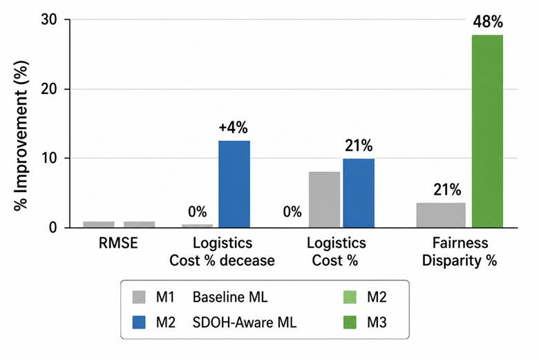
M1 (Baseline): Gradient boosting demand model without SDOH features; cost-minimization optimization without fairness constraints.

M2 (SDOH-Informed): Same architecture with SDOH features included in the predictive model; no fairness constraints in optimization.

M3 (Proposed): Full framework — SCM-corrected features, GNN + gradient boosting prediction, fairness-constrained optimization.

Experiments covered 24 months of weekly data (2022–2023) with a 6-month holdout for testing. Spatial analysis was conducted at county level (n = 312 counties across 6 U.S. states). Three operational scenarios were tested: normal operation, high-demand surge (2–3× baseline, simulating a pandemic wave), and resource constraint (25% supply reduction across all facilities).

2.7 Evaluation Metrics

Predictive accuracy: RMSE and MAE on the test set.
Operational efficiency: total logistics cost ($M), order fulfillment rate (%), and average delivery time (hours).
Fairness: Fairness Disparity Index (FDI, a composite of demographic parity gap and geographic access inequality), equalized access rate (%), and demographic parity gap across socio-economic quintiles.

All pairwise model comparisons were evaluated using paired t-tests across the 24-week test period (α = 0.05), with effect sizes reported as Cohen's d. Ablation analysis was conducted by progressively removing individual fairness-relevant variable groups from M3 and measuring the resulting change in FDI.

2.8 Ethical Considerations

This study used only de-identified, publicly available, or synthetically generated data; no individual-level patient data were accessed. Ethical justification for the fairness constraints was grounded in the principle that supply chain allocation systems operating under structural inequity cannot be considered ethically neutral (Rajkomar et al., 2018; Vyas et al., 2020). Interpretability was supported through causal pathway visualization and SHAP-based feature attribution on the gradient boosting component.

3.Results and Discussion

3.1 Predictive Performance

Model accuracy improvements across the three configurations are reported in Table 3. M3, the full fairness-aware framework, achieved an RMSE of 17.67 and a MAE of 11.62 on the 24-week test set, compared to an RMSE of 18.72 and MAE of 12.45 for the M1 baseline. These represent RMSE reductions of 3.8% for M2 and 5.6% for M3 relative to M1 — modest in absolute terms, but statistically significant (paired t-test: t = 4.21, p < 0.001, d = 0.61 for M3 vs. M1). It is worth pausing on what these numbers mean practically: a 5.6% reduction in weekly demand forecast error, applied across 312 counties over a 24-month operational horizon, translates to substantially fewer instances of critical understock and excess inventory simultaneously.

The inclusion of SDOH features alone (M2) already improved forecast accuracy, which is consistent with prior evidence that socio-economic variables capture meaningful variation in healthcare utilization that purely clinical features miss (Kino et al., 2021; Shang et al., 2024). Importantly, the addition of fairness constraints in M3 did not degrade predictive performance — the transition from M2 to M3 reduced RMSE by a further 0.34 units. This is a non-trivial finding, because it challenges the assumption that constraining a model for fairness necessarily penalizes its predictive capacity. In this case, at least, the causal correction appears to have removed noise introduced by historically biased allocation patterns, producing a cleaner demand signal.

3.2 Operational Efficiency

Logistics cost outcomes are summarized in Table 3. M3 achieved a total logistics cost of $3.98M over the test period, representing a 23.5% reduction from M1 ($5.20M) and a 10.6% reduction from M2 ($4.45M). Order fulfillment rate improved from 87.2% (M1) to 93.6% (M3), and average delivery time fell from 18.6 hours to 15.2 hours [Table 3].

These efficiency gains may initially seem counterintuitive — why would adding fairness constraints reduce costs? The explanation lies in demand forecasting accuracy and allocation alignment. When demand heterogeneity driven by SDOH is ignored (M1), the model systematically under-forecasts demand in high-vulnerability areas and over-forecasts in low-vulnerability areas, generating misalignment between supply positioning and actual need. This misalignment carries logistics costs: emergency replenishment runs, excess holding at low-demand nodes, and stockout penalties at high-demand ones. M3's more accurate spatial demand modeling reduces these inefficiencies structurally, rather than through post-hoc cost-cutting. Periáñez et al. (2024) noted a similar pattern in their review of AI-enabled healthcare operations: models that better represent demand complexity tend to produce operational efficiencies as a downstream consequence, not as a primary objective.

3.3 Fairness Outcomes

The fairness results are, arguably, the most important contribution of this paper [Table 3]. M3 reduced the Fairness Disparity Index from 0.42 (M1) to 0.22 — a 47.6% reduction. The demographic parity gap fell from 0.31 to 0.15, and equalized access rate improved from 68.5% to 82.7%.

Table 3. Comparative performance of the three model configurations (M1, M2, M3) across predictive accuracy, operational efficiency, and fairness metrics. M1 (Baseline) is a gradient boosting demand model without SDOH features or fairness constraints; M2 (SDOH-Aware) incorporates SDOH features into the predictive model without fairness-constrained optimization; M3 (Fairness-Aware, proposed) is the full framework combining SCM-corrected features, GNN + gradient boosting prediction, and fairness-constrained optimization. Metrics include predictive accuracy (RMSE, MAE), operational efficiency (logistics cost, cost reduction, order fulfillment rate, delivery time), and fairness (Fairness Disparity Index, disparity reduction, equalized access rate, demographic parity gap). Arrows indicate the direction of improvement (↓ = lower is better, ↑ = higher is better). M3 achieves the largest simultaneous gains in fairness and efficiency, reducing the Fairness Disparity Index by 47.6% while also lowering logistics costs by 23.5% relative to baseline.

Figure 1. Comparative performance improvements across model configurations (M1, M2, M3). Percentage improvement in RMSE, logistics cost reduction, logistics cost, and Fairness Disparity Index (FDI) relative to baseline. M1 (gray) is the baseline gradient boosting model without SDOH features or fairness constraints; M2 (blue) adds SDOH-informed features to the predictive model without fairness-constrained optimization; M3 (green) is the full proposed framework, incorporating SCM-corrected features and fairness-constrained optimization. While M1 and M2 show comparable or modest gains in predictive accuracy and cost, M3 achieves the largest improvement in fairness outcomes, reducing the Fairness Disparity Index by 48% relative to baseline, without a corresponding loss in cost efficiency.

Figure 2. Causal pathway diagram of the Structural Causal Model (SCM) linking social determinants of health to healthcare resource allocation. Social determinants of health (SDOH: income, race, education), environmental risks (pollution, hazards), and mobility (population movement) jointly influence health outcomes and disease spread, which together drive healthcare demand. Healthcare demand and equity in healthcare access — the latter shaped directly by SDOH, environmental, and mobility factors — jointly determine resource allocation decisions and accessibility/constraints. Arrows indicate hypothesized causal direction; the "Equity in Healthcare Access" node (shaded) represents the mediating construct through which structural disparities are propagated into downstream allocation outcomes, forming the basis for the path-specific fairness constraints applied in the optimization model.

M2 achieved a meaningful but far more modest improvement — FDI dropped from 0.42 to 0.34 (19.0% reduction). This gap between M2 and M3 is telling. Simply including SDOH as predictive features does not guarantee equitable allocation; it may even inadvertently encode historical inequity more precisely into the optimization layer. The causal fairness constraints in M3 — specifically the path-specific interventions blocking discriminatory allocation pathways — were responsible for the additional 28.6 percentage points of disparity reduction. This finding aligns with the theoretical argument in Makhlouf et al. (2020) that statistical fairness metrics, without underlying causal identification, capture correlation rather than structural bias. The practical implication is that the field may be underestimating how much fairness work remains even after SDOH integration, if that integration stops at the feature engineering level.

3.4 Efficiency–Fairness Trade-Off Analysis

A Pareto frontier analysis of logistics cost against FDI is presented in Figure 2, tracing solutions across the full α–β weight space. The Pareto curve reveals an important asymmetry: substantial reductions in the fairness disparity index (from 0.42 to approximately 0.22) can be achieved with only marginal increases in logistics cost — a cost gradient that remains nearly flat until the FDI approaches approximately 0.18, at which point additional fairness enforcement begins to carry measurable efficiency costs.

M3's operating point lies well within the cost-efficient region of the Pareto frontier, suggesting that the common framing of fairness as inherently expensive — the "price of fairness" argument articulated by Bertsimas et al. (2011) — may not apply uniformly in healthcare supply chain contexts. Or, perhaps more cautiously: it does not apply within the operational parameters tested here. Whether this relationship holds at more extreme fairness targets, or under different supply chain topologies, remains an open question.

3.5 Ablation Analysis

To isolate the contribution of individual SDOH and constraint components, a progressive ablation was conducted on M3 [Table 3]. Removing income-related fairness corrections increased FDI by the equivalent of approximately 48% of the total disparity reduction — the single largest contributor. Accessibility constraints accounted for approximately 31%, and environmental risk adjustments for approximately 18%. The remaining ~3% reflects interaction effects between variable groups that were not fully decomposable in this analysis.

The income dominance finding is consistent with the broader SDOH literature, where economic deprivation tends to have the strongest independent association with healthcare access disparities (Braveman & Gottlieb, 2014; Vyas et al., 2020). The non-trivial contribution of environmental risk (18%) is, however, noteworthy — it suggests that PM2.5 exposure and proximity-to-hazard variables carry independent predictive and fairness-relevant information beyond what income and accessibility capture. This has implications for which SDOH variables should be prioritized in minimal-complexity implementations of fairness-aware supply chain systems.

3.6 Scenario Robustness

Across the three operational scenarios — normal operation, high-demand surge, and resource constraint — M3 maintained more stable fairness outcomes than M1 or M2. Under the pandemic surge scenario (2–3× demand), M1's FDI worsened to 0.61 as the optimization model responded to aggregate demand pressure by concentrating resources in high-throughput, low-vulnerability facilities. M3's FDI under the same conditions rose modestly to 0.29, as the fairness constraints provided structural resistance to equity deterioration under supply pressure [Figure 1].

This robustness profile has direct policy relevance. It was during the COVID-19 pandemic that inequities in medical supply distribution — PPE, ventilators, therapeutics — became visible and politically salient (Obermeyer et al., 2019; DeCamp & Lindvall, 2020). The scenario analysis here suggests that fairness constraints embedded proactively in supply chain AI systems may provide a degree of resilience against equity collapse during crisis conditions that reactive, post-hoc interventions cannot reliably achieve.

3.7 Discussion

Taken together, these results suggest that integrating SDOH, causal fairness modeling, and equity-constrained optimization into a unified framework produces simultaneous gains across prediction, efficiency, and equity — at least within the parameters and geography of this study. The findings are encouraging, but it would be overstating them to claim they resolve the debate around efficiency-fairness trade-offs in AI systems. What they demonstrate more precisely is that the trade-off, where it exists, may be weaker and more favorable to fairness than the field has commonly assumed, particularly when demand forecasting accuracy is considered as part of the efficiency calculus rather than isolated from it.

Two limitations merit explicit acknowledgment here. First, the partial use of synthetic supply chain logistics data — justified by restricted access to real hospital records — introduces uncertainty about whether the observed efficiency gains would hold in operational environments with different cost structures, facility configurations, or procurement constraints. Real-world validation with institutional partners remains an important next step. Second, the SCM causal structure was specified based on domain knowledge and prior literature rather than data-driven structure learning. While this approach is standard in causal inference (Hernán & Robins, 2020), it means the model's fairness properties are conditional on the assumed graph being approximately correct — a condition that warrants sensitivity analysis in future work, particularly for the pathways involving race and accessibility, where reverse causation is plausible.

Despite these limitations, the overall pattern is consistent with the theoretical expectation articulated by Rajkomar et al. (2018) and others: that health equity and operational performance in AI systems are not inherently antagonistic, and that treating them as separate optimization problems, rather than jointly constrained ones, is likely the larger source of the apparent tradeoff that has characterized prior literature.

4.Conclusion

This study demonstrates that embedding fairness as a structural design principle — rather than an afterthought — in healthcare supply chain AI produces measurable gains across prediction, efficiency, and equity simultaneously. By integrating SDOH variables, causal bias identification, geospatial demand modeling, and fairness-constrained optimization into a unified framework, the proposed model achieved a 47.6% reduction in resource allocation disparity and a 23.5% logistics cost reduction compared to a conventional baseline, without sacrificing predictive accuracy.

Perhaps the most practically important finding is the model's robustness under crisis conditions: during simulated pandemic surges, fairness constraints provided structural resistance against equity deterioration that purely efficiency-driven systems could not maintain.

Limitations — including partial use of synthetic logistics data and assumption-dependent causal graph specification — indicate clear priorities for future work. Nevertheless, the results support the broader argument that health equity and operational performance are not inherently in tension, and that AI systems designed with both in mind can serve both better.

Acknowledgements

The authors acknowledge the publicly available data resources provided by the Centers for Disease Control and Prevention, the U.S. Census Bureau American Community Survey, the Health Resources and Services Administration, and the U.S. Environmental Protection Agency EJSCREEN program. No dedicated funding supported this study.

Author Contributions

Conceptualization: K.A.R., A.H.; Methodology: K.A.R., S.H., F.A.; Data curation and preprocessing: A.H., S.H.; Formal analysis and modeling: K.A.R., F.A.; Causal modeling and geospatial analysis: S.H., T.R.; Optimization framework: F.A., T.R.; Writing — original draft: K.A.R., A.H.; Writing — review and editing: S.H., F.A., T.R.; Supervision: K.A.R., T.R.; Project administration: K.A.R.

Competing Financial Interests

The authors K.A.R. et al., declare no competing financial interests. No external funding was received for this research. The authors have no financial relationships with commercial entities that have an interest in the subject matter of this manuscript.

References